Monday, November 30, 2015

green01 格林公式(图 3)的意义在于: 一维的定积分通过牛顿---莱布尼茨公式得到了完满的解决,等于不定积分原函数的两个取值之差。不定积分是一个函数的全体原函数,是一个函数族(函数的集合);

定积分和不定积分的区别


这两者是从不同角度定义的不同概念。
不定积分是一个函数的全体原函数,是一个函数族(函数的集合);
定积分是与函数有关的一个和式的极限,是一个实数。
从概念而言,这两者是完全不同的、毫无关系的,或者说是风马牛不相及的。
但是牛顿-莱布尼兹公式却把它们联系起来,这就是这两位先驱者的伟大之处,虽然在今人看起来并没有多少深奥,倒反而有人会把这两个概念混淆在一起。如果当初这两个概念也那么容易相混的话,大概等不到牛顿出生,微积分早被创立了。
牛顿-莱布尼兹公式告诉我们,定积分那个极限,等于被积函数的原函数在积分区间右端点的值减去左端点的值,定积分也就与原函数有了联系,定积分之所以叫定积分大概也是因为这个原因。但是取这个名也有副作用,因为不定积分比定积分只多了一个“不”字,一些人就认为它们是一样的或者是稍有区别的,这大概也是今天这个问题被提出的原因。
建议学习高等数学的同学们,不要问不定积分与定积分有什么区别,而是把它们作为两个完全不同的概念分别学习好,再也不要搞混在一起。

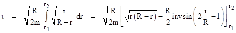
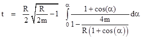
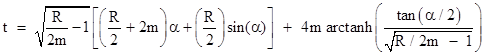
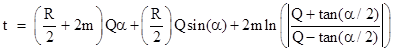
曲线积分的物理意义 [引用和转载请标明本文 CU blog 出处]         定积分的求解---牛顿.拉布尼茨公式有什么几何意义? 简单的说,因为 F(b)-F(a)在几何上是 f(x) 的原函数 F(x)在 y 轴上的线段长度,那么这个长度如何表示呢? F(b)-F(a)可以写成在区间[a,b]上面的累 加 Sigma(F'(x)*delta(x)),那么这个 Sigma 就是 f(x)的定积分了。反向构造的方法联系了不定积分和 定积分(图 1)。         太抽象了,举个有物理含义的例子(图 2)。 1. 假设 x/y 平面是一个力场,一个质点在立场中受力,它受的力在 x 轴方向方向的投影值,恰好等于它 的 y 坐标(力的正负代表方向)。 2.那么这个例子沿着曲线 y^2=x,从(1,-1)移动到(1,1),立场对它作了多少功?          我们可以画出一个图形,粒子在 y 的负半平面受的力总是向左的(负号),在 y 的正半平面受的力总 是向右的,所以立场一直在 x 轴方向对例子做正的功。做功的积分式子分为两个部分,(1,-1)到(0,0)的过 程是 S[x,1,0],dx 是负数,力 y=x^0.5 也是负数,负负得正。所以做的总功=2*S[x,0,1](x^0.5), 这个解求很简单了。那么如果立场还有一个 y 方向呢? 叠加的结果就是 2*S[x,0,1]+S[y,-1,1],写成积 分式子,就是对于坐标的曲线积分。
            格林公式(图 3)的意义在于:         一维的定积分通过牛顿---莱布尼茨公式得到了完满的解决,等于不定积分原函数的两个取值之差。 那么格林公式的意义呢? 曲线积分,分成 dx 和 dy 的两部分分别证明。考虑凸面曲线的情况,因为其他情 况可以分解为若干个凸面曲线的情况。例如要证明格林公式中关于 dy 的部分,就可以看作很多条平行于 x 轴的线穿过被积分的曲线,其中每一条直线和曲线交与两点,靠近 y 轴左半平面的点记做 Q1,靠近 y 轴 右半平面的点记做 Q2,那么根据曲线积分的正向定义,逆时针方向,Q1 点的微元 dy 是正的,Q2 点的 微元 dy 是负的。然后微元的和就是 Q1*dy+Q2*(-dy)=(Q1-Q2)dy。好了,Q1-Q2 又是多少呢? 由牛 顿莱布尼茨公式得到它是 Q2-Q1 这条线段上 Q'(x)的积分和。那么积分和的和就是一个 2 重积分。         用一个黎曼球面我们把|z|从 0 到无穷大的所有的矢量影射到了一个南北极的球面上面(彩图右上), 无穷的数域变成了有穷的数域。微分方程变成指数方程,纯为粉方程类似线形代数的方程组由通解和特解
组成解系;指数变成拉伸和旋转,平面几何的问题变成解析几何的问题。举个例子,如何判断两条直线是 否垂直,那么 z1(角度 Theta1)和 z2(角度 Theta2)互相垂直相当于 z1 和 z2 之间的夹角=正负 90 度。 由于复数的乘法包含了角度的相加,那么 z2 的共轭矢量角度就是-Theta2。它们两个相乘的结果矢量角就 是 Theta1-Theta2,如果这个角度是 90 度,那么 z1*z2'就应该是一个纯虚数,反之,z1*z2'是个纯虚 数,就说明 z1 和 z2 垂直。所谓的"虚数"并不是不存在,而是它的值在实数轴 x 上面的投影总是 0。那么 写出来就是a+bi与c+di正交的充要条件就是ac+bd=0----看起来像是线形代数里面的[a,b]与[c,d] 互 相正交的充要条件是矢量点乘=0。复数,确实是用线形代数的方式在研究高等数学,把函数的研究统一到 了解析几何。这里,代数和几何没有区别。         再举一个例子,平面几何的命题(图 4):一个三角形 AB=AC,AB 上有线段 mn,AC 上有线段 jk, 长度 mn=长度 jk,证明 mj 的中点 x 和 nk 的中点 y,连线垂直于 BC。这道题如果用初等数学平面几何 的性质,脑袋破了都很难证明,因为平面几何的定理是用语言表述的某种性质,证明的过程也是和人对图
形的感性认识密切相关,例如垂直平分线,等腰三角形,这些自然语言的概念用起来太费劲,而且必须结 合图形本身来使用。OK,用复数来证明,使用一个形式语言的演算系统: 1. 假设 AB 是实数轴,AC 是和 AB 夹角为 a 的向量,那么假设等腰边长为 l ,那么
AB=l,AC=l(cosa+isina),BC=AC-BC=l(cosa-1 +isina)。 2. 假设 mn 和 jk 的长度为 r,m=M+0i,j=M(cosa+isina),那么 n=M+r,k=(M+r)(cosa+isina)。 3. mj 的中点就是 d1=(m+j)/2,nk 的中点就是 d2=(n+k)/2,两点之间的连线的方向矢量 f1=d2-d1=(n+k-m-j)/2 4. BC 的共轭矢量 f2=l(cosa-1-isina) 5. f1*f2,去掉实系数=(cosa+1+isina)(cosa-1-isina),实部=cosa^2-1+sina^2=0,所以是个纯 虚书,根据上例的结果,f1 和 f2 垂直,证毕。         再举一个证明题:平行四边形对角线的平方和=相邻对角线平方和的两倍。那么设四边形的两条边 是矢量 z1 和 z2 ,那么|z1+z2|^2+|z1- z2|^2=(z1+z2)(z1'+z2')+(z1-z2)(z1'-z2')=2z1z1'+2z2z2'=2(|z1|^2+|z2|^2)得证。复数的函 数(复变函数)往往具有对称性的性质。如果 f(z)=a0+a1z^1+...+anz^n=X+Yi,那么可以证明, f(z')=X- Yi。有什么作用吗? 如果函数 f(z)=0 有解 a+bi,那么 a-bi 也是解(显然因为 X=Y=0)。复数 更重要的特征是矢量的方向性。一个直线过 z1,z2 的端点,那么方向就是 M(z2-z1),直线方程就可以写 成点法式: z1+M(z2-z1)=Mz2+(1-M)z1。         朱力斯·华纳有一幅很著名的画叫做"神秘的岛屿"(彩图左上),这个画的内容看起来是个探险的小 岛,但是把一个圆柱形的镜面放到画的中央,人们惊奇的发现其实这是作者的自画像。如果这幅洋洋洒洒 的油画是代表了实数的问题,那些无穷无尽的无比复杂的现实问题,那么这个圆柱形的镜子就是"复数"这 样一个发明,它把无穷复杂的问题变成了有穷范围内能表达的问题。由于一一映射的存在,实数域难以解
决的问题通过映射和等效,在复数域通常能得到简单的解答,再映射回实数域,便是问题的解。例如著名 的莫比乌斯变换(彩图右下)。
        需要很好的考虑几个问题: 1. 我们在把可积函数变成傅立叶级数的时候,曾经强调过,每个分量之间由于是三角函数族的成员,所以 构成正交关系,所以显然,分量之间没有重叠,展开式显然唯一。那么对于泰勒级数和复分析当中的洛朗 级数而言,函数的幂级数展开式是否是唯一的? 我们主要到没有任何条件限制规定展开分量之间必须构成 正交关系。正交性并不必要,基不需要正交性。 z 和 z^2 线性无关(注意是“线性”)因为不存在 c1 和 c2\in R,使得 c1*z + c2*z^2=0, 对于所有的 z 属于 R 都成立(z 是变量,可以任意取)。严格的说,“幂分量” 不需正交,仅要线性无关即可。反证法,我们假设幂级数的分量之间是线形相关的,也就是存在常数 k1-kn 使得(k1(1 是角标))k1x+k2x^2+k3x^3+...+knx^n =0。我们又知道前面这个方程,在复数域中仅 有 n 个解,即 0 点仅有 n 个。故只有 k1=k2=....=kn 左端才恒为 0(对于任意的 z),这就是线性无关的 条件,n 任意个,即无穷个 x^i 都线性无关。当然这里线性空间是一个函数空间,其实 x,x^2,...构成其 一个基----所以 k1-kn 都是 0, {z^n}构成的分量,是个线性无关的集合(两两之间)。 2. 为什么洛朗级数(彩图红色圆环)里面会有复数次幂? 我们去掉不解析的点,就得到了一些列圆环,这个 圆环上作闭合路径包围一定的面积,就是里外两条曲线,外围曲线就是洛朗技术的 n>=-1 的幂次项,内 围曲线是反方向的环绕无穷原点(很奇怪吗? 只要把 z 平面映射到黎曼球面上,就会得到这个结论!),是一 个负数的积分结果,它的收敛半径相反,我们把 z 用 z 的倒数来代替,就得到了和前半部分几乎一样的表 达式。所以洛朗级数的形式是 Sigma 从 n=负无穷到正无穷的形式(完备)。特别的,如果圆环是圆饼,那 么内环等于是不存在或者收缩到了一个点,也就是 n<-1 的那些负数次幂不存在了,函数解析,得到洛朗 级数等于泰勒级数的结论。实变函数可以展开成泰勒级数----本质的意义不在于泰勒级数的导数项,而是 在于,函数可以展开成自变量所表达的一个幂级数求和表达式,这个有点像离散结构里面的 P 问题。那么 对于复数,因为解释函数的方向导数有无数个,所以无法直接表示成泰勒级数,但是仍然可以写成幂级数 求和的形式----洛朗级数,同时,可以把泰勒级数看成洛朗级数在实轴方向上投影的特例。当然,这个时 候的幂级数系数不能再用导数来求了(切线逼近法),而是使用一个积分。Taylor 级数可以看作 Lorent 级 数的特例。泰勒级数有个收敛域(x-x0,x+x0)和收敛条件 x 附近连续且可导。我们放到复数平面上来,收 敛域就是一个圆,在 x 点处解析。但是如果不满足解析条件呢? 对于一个复变量函数 f(z)来说,如果它在 某点是全纯的(解析的),则它一定有 Taylor 级数,        复平面的点和黎曼圆的点一一对应,所以所有的直线在无穷远处必定相交,哪怕是平行线----这就是 黎曼几何不同于欧式几何的一个地方。无穷远的点集被映射成为 N 点--->于是留数基本定理,所有奇异点 的留数和=0 就很好理解了: 流体从各个有限奇异点流出,汇聚到无穷远的奇异点,流入流出的总和=0。 同理,如果黑洞是一个奇异点,那么当黑洞需要喷发的时候,喷发的方向显然是阻力小的方向,和黑洞 周围的圆盘垂直的法向量。为什么复变函数里面会有那么怪异的柯西积分公式? 实际上还是从格林公式推 导出来的,解析函数对于某点的围线积分等于围绕 z0 点本身的无穷小圆的积分,这个性质说明了解析函 数的 2 维积分中值定理: f(z)可以从围线的积分中值来求,反过来,一个积分可以看成是 f(z)的洛朗级数 展开的-1 次项,于是 1 元积分学当中的许多问题就借助 2 元复变函数得以解决了。       格林公式是把 1 维的围线积分和 2 重积分联系起来了,而复数则推广了,一维的围线积分(被积函数 有不可导点)还可以等价于被积函数本身的取值。这真是一个简单而且美的结论----f(z)*2Pi*i 的取值等于 围绕着 z,f(w)/(z-w)做一圈封闭的曲线积分----当然和曲线的形状无关。f(z)和非 z 点的 f(w)被这个方 程式统一了起来,多么奇妙的一件事情。如果把 z 看成圆点(黑洞),那么就是圆点这个黑洞的能量可以通 过围绕这个黑洞的一个曲线上的矢量积分来判定,黑洞变得可以测量了。另一方面,这个方程给出了解析 的函数,各个点之间的某种相关性。一个点可以用其他的点集的某种积分来表示。    
(Abel 整理于网络,非原创)


化学基本概念反映化学物质的本质属性,是化学的基础。明确概念的内涵与外延,是正确把握知识的要素,也是正确判断和推理的基础,因此在概念的教学中,让学生掌握、运用概念,尤为重要。同位素、同素异形体、同系物、同分异构体和同一种物质等化学中几个经常用到的概念,也是一些同学经常混淆的概念,下面就这几个概念的区别加以详细的说明。
           
对于同位素、同素异形体、同系物和同分异构体这四个概念,学习时应着重从其定义、对象、化学式、结构和性质等方面进行比较,抓住各自的不同点,从而理解和掌握。这几个概念都表明了事物之间的关系,下表列出了比较了它们的异同:


同位素
同素异形体
同系物
同分异构体
定义
质子数相同,中子数不同的原子(核素)
由同一种元素组成的不同单质
结构相似,分子组成相差一个或若干个CH2基团的物质
分子式相同,结构不同的化合物
对象
原子
单质
化合物
化合物
化学式
元素符号表示不同,如、、
元素符号表示相同,分子式可以不同,如O2和O3
不同
相同
结构
电子层结构相同,原子核结构不同
单质的组成或结构不同
相似
不同
性质
物理性质不同,化学性质相同
物理性质不同,化学性质相同
物理性质不同,化学性质相似
物理性质不同,化学性质不一定相同

说明:

1、同位素的对象是原子,在元素周期表上占有同一位置,化学性质基本相同,但原子质量或质量数不同,从而其质谱行为、放射性转变和物理性质(例如在气态下的扩散本领)有所差异。

2、同素异形体的对象是单质,同素异形体的组成元素相同,结构不同,物理性质差异较大,化学性质有相似性,但也有差异。如金刚石和石墨的导电性、硬度均不同,虽都能与氧气反应生成CO2,由于反应的热效应不同,二者的稳定性不同(石墨比金刚石能量低,石墨比金刚石稳定)。
 
同素异形体的形成方式有三种:
 
 (1)组成分子的原子数目不同,例如: O2和O3 。
  (2)晶格中原子的排列方式不同,例如:金刚石和石墨。
    (3)晶格中分子排列的方式不同,例如:正交硫和单斜硫(高中不要求此种)。

注意:同素异形体指的是由同种元素形成的结构不同的单质,如H2和D2的结构相同,不属于同素异形体。

3、同系物的对象是有机化合物,属于同系物的有机物必须结构相似,在有机物的分类中,属于同一类物质,通式相同,化学性质相似,差异是分子式不同,相对分子质量不同,在组成上相差一个或若干个CH2原子团,相对分子质量相差14的整数倍,如分子中含碳原子数不同的烷烃之间就属于同系物。

   (1)结构相似指的是组成元素相同,官能团的类别、官能团的数目及连接方式均相同。结构相似不一定是完全相同,如CH3CH2CH3和(CH3)4C,前者无支链,后者有支链,但二者仍为同系物。
(2)通式相同,但通式相同不一定是同系物。例如:乙醇与乙醚它们的通式都是CnH2n+2O,但他们官能团类别不同,不是同系物。又如:乙烯与环丁烷,它们的通式都是CnH2n,但不是同系物。
(3) 在分子组成上必须相差一个或若干个CH2原子团。但分子组成上相差一个或若干个CH2原子团的物质却不一定是同系物,如CH3CH2Br和CH3CH2CH2Cl都是卤代烃,且组成相差一个CH2原子团,但二者不是同系物。
(4)同系物具有相似的化学性质,物理性质有一定的递变规律,如随碳原子个数的增多,同系物的熔、沸点逐渐升高;如果碳原子个数相同,则有支链的熔、沸点低,且支链越对称,熔、沸点越低。如沸点:正戊烷>异戊烷>新戊烷。同系物的密度一般随着碳原子个数的增多而增大。

4、同分异构体的对象是化合物,属于同分异构体的物质必须化学式相同,结构不同,因而性质不同。具有“五同一异”,即同分子式、同最简式、同元素、同相对原子式量、同质量分数、结构不同。属于同分异构体的物质可以是有机物,如正丁烷和异丁烷;可以是有机物和无机物,如氰酸铵和尿素;也可以是无机物,如[Pu(H2O)4]Cl3和[Pu(H2O)2Cl2]·2H2O·Cl。

在有机物中,很多物质都存在同分异构体,中学阶段涉及的同分异构体常见的有以下几类:
(1)碳链异构:指碳原子之间连接成不同的链状或环状结构而造成的异构。如C5H12有三种同分异构体,即正戊烷、异戊烷和新戊烷。

(2)位置异构(官能团位置异构):指官能团或取代基在在碳链上的位置不同而造成的异构。如1—丁烯与2—丁烯、1—丙醇与2—丙醇、邻二甲苯与间二甲苯及对二甲苯。

(3)类别异构(又称官能团异构):指官能团不同而造成的异构,如1—丁炔与1,3—丁二烯、丙烯与环丙烷、乙醇与甲醚、丙醛与丙酮、乙酸与甲酸甲酯、葡萄糖与果糖、蔗糖与麦芽糖等。

(4)其他异构方式:如顺反异构、对映异构(也叫做镜像异构或手性异构)等,在中学阶段的信息题中屡有涉及。

各类有机物类别异构体情况:

⑴ CnH2n+2:只能是烷烃,而且只有碳链异构。如CH3(CH2)3CH3、CH3CH(CH3)CH2CH3、C(CH3)4

⑵ CnH2n:单烯烃、环烷烃。


如CH2=CHCH2CH3、CH3CH=CHCH3、CH2=C(CH3)2、           、

⑶ CnH2n-2:炔烃、二烯烃、环烯烃。如:CH≡CCH2CH3、CH3C≡CCH3、CH2=CHCH=CH2、

⑷ CnH2n-6:芳香烃(苯及其同系物)。如:           、          、

⑸ CnH2n+2O:饱和脂肪醇、醚。如:CH3CH2CH2OH、CH3CH(OH)CH3、CH3OCH2CH­3

⑹ CnH2nO:醛、酮、环醚、环醇、烯基醇。如:CH3CH2CHO、CH3COCH3、CH2=CHCH2OH、                  
                      、          、

⑺ CnH2nO2:羧酸、酯、羟醛、羟基酮。如:CH3CH2COOH、CH3COOCH3、HCOOCH2CH3、
HOCH2CH2CHO、CH3CH(OH)CHO、CH3COCH2OH
  
 ⑻ CnH2n+1NO2:硝基烷、氨基酸。如:CH3CH2NO2、H2NCH2COOH
⑼ Cn(H2O)m:糖类。如: C6H12O6:CH2OH(CHOH)4CHO、CH2OH(CHOH)3COCH2OH

C12H22O11:蔗糖、麦芽糖。

例1、下列各组物质中,两者互为同分异构体的是(      )。


①CuSO4?3H2O和CuSO4?5H2O     ②NH4CNO和CO(NH2)2


③ C2H5NO2和NH2CH2COOH       


 ④[Pu(H2O)4]Cl3和[Pu(H2O)2Cl2] ?2H2O?Cl


A、①②③       B、②③④       C、②③        D、③④


解析:同分异构体是分子式相同,但结构不同。CuSO4?3H2O和CuSO4?5H2O组成就不同,不是同分异构体;NH4CNO和CO(NH2)2分子式相同,二者结构不同,互为同分异构体;C2H5NO2和NH2CH2COOH,前者是硝基化合物,后者是氨基酸,分子式相同,属于类别异构;[Pu(H2O)4]Cl3和[Pu(H2O)2Cl2] ?2H2O?Cl,前者表示四个水分子直接和Pu相结合,后者中是两分子的水和两个氯离子与Pu相结合,所以结构不同,互为同分异构体。正确选项为B。


例2、下列各组物质,其中属于同系物的是(      )。


(1)乙烯和苯乙烯      (2)丙烯酸和油酸      (3)乙醇和丙二醇 


(4)丁二烯与异戊二烯  (5)蔗糖与麦芽糖


 A.(1)(2)(3)(4)          B.(2)(4)


 C.(1)(2)(4)(5)          D.(1)(2)(4)


解析:同系物是指结构相似,即组成元素相同,官能团种类、个数相同,在分子组成上相差一个或若干个


CH2原子团,即分子组成通式相同的物质。乙烯和苯乙烯,后者含有苯环而前者没有;丙烯酸和油酸含有的官能


团都是双键和羧基,而且数目相同所以是同系物;乙醇和丙二醇官能团的数目不同;丁二烯与异戊二烯都是共


轭二烯烃,是同系物;蔗糖和麦芽糖是同分异构体而不是同系物。正确选项为B。


例3、有下列各组微粒或物质:
                                                              CH3
A、O2和O3          B、C和C        C、CH3CH2CH2CH3和 CH3CH2CHCH3
       H           Cl                                      CH3
D、Cl—C—Cl和Cl—C—H           E、CH3CH2CH2CH3和CH3—CH—CH3
       H           H
(1)                组两种微粒互为同位素;
(2)                组两种物质互为同素异形体;
(3)                组两种物质属于同系物;
(4)                组两物质互为同分异构体;
(5)                组两物质是同一物质。

解析:这道题主要是对几个带“同字”概念的考查及识别判断能力。A项为都由氧元素形成的结构不同的单质,为同素异形体。B项为质子数相同,中子数不同的原子,属于同位素。C项均为烷烃结构,分子组成上相差一个CH2原子团,属于同系物。D项均为甲烷的取代产物,因而是立体结构,是同种物质。D项的分子式相同,结构不同(碳链异构),是同分异构体。
正确选项为:(1)B    (2)A   (3)C    (4)E    (5)D
例4.如果定义有机物的同系列是一系列结构简式符合: (其中n=0、1、2、3……)的化合物。式中A、B是任意一种基团(或氢原子),w为2价的有机基团,又称为该同系列的系差。同系列化合物的性质往往呈现规律性变化。下列四组化合物中,不可称为同系列的是:
  A.CH3CH2CH2CH3       CH3CH2CH2CH2CH3        CH3CH2CH2CH2CH2CH3
  B.CH3CH=CHCHO     CH3CH=CHCH=CHCHO     CH3(CH=CH)3CHO
  C.CH3CH2CH3        CH3CHClCH2CH3        CH3CHClCH2CHClCH3
  D.ClCH2CHClCCl3     ClCH2CHClCH2CHClCCl3    ClCH2CHClCH2CHClCH2CHClCCl3

解析:此题是95年全国高考题,也是一个信息题,信息中给出了一个新的概念同系列。在课堂上我们学习过同系物这一概念。这就形成了两个非常相近的概念,需要我们在理解新信息的基础上,进行对比、辨析,然后运用解题。同系物是指结构相似,在分子组成上相差一个或若干个CH2原子团的物质。而同系列是指结构相似,在结构上相差一个或若干个重复结构单元的物质。据此可迅速作出判断,正确选项为C。
练习:

1.在热核反应中没有中子辐射,作为能源时不会污染环境。月球上的储量足够人类使用1000年,地球上含量很少。和两者互为(    )
A.同素异形体    B.同位素     C.同系物      D.同分异构体
解析:和的质子数相同,中子数不同,二都均为原子,互为同位素。答案: B

2.美国和墨西哥研究人员将普通纳米银微粒分散到纳米泡沫碳(碳的第五种单质形态)中,得到不同形状的纳米银微粒,该纳米银微粒能有效杀死艾滋病病毒(HIV-1)。纳米泡沫碳与金刚石的关系是学科网(Zxxk.Com)学科网
A.同素异形体       B.同分异构体        C.同系物          D.同位素学科网(Zxxk.Com)学科网

解析:因纳米泡沫碳是碳的第五种单质形态,而金刚石也是碳的一种单质同体,所以二者是由同种元素形成的结构不同的单质,故为同素异形体。答案:A

3.下列各对物质中属于同分异构体的是(       )。
A.C与C                         B.O2与O3
解析:A是同位素,B是同素异形体,C是同一物质,D是同分异构体。答案:D

4.下列各组物质中,互为同系物的是(       )。                                                                         
A.    —OH与    —CH3                B. HCOOCH3 与CH3COOC3H7                             
C.    —CH=CH2 与CH3—CH=CH2       D. C6H5OH与C6H5CH2OH  

解析:A项二者相差一个氧原子,不是同系物。B项均为酯,结构相似,又分子组成上相差一个CH2原子团,属于同系物。C项不是同一类别的有机物,结构不相似,不是同系物。D项的C6H5OH是苯酚,C6H5CH2OH是苯甲醇,不是同一类别的,结构不相似,不是同系物。答案: B

5.下列各组物质中一定互为同系物的是(       )。
A.C3H8、C8H18    B. C2H4、C3H6      C. C2H2、C6H6     D. C8H10、C6H6

解析:A项均为烷烃,分子组成上相差CH2原子团,是同系物。B项不一定互为同系物,当二者都是烯烃时,是同系物;当C3H6是环丙烷时,不是同系物。同理,C项结构不相似,不是同系物。D项可以是不同的类别,不一定是同系物。答案: A

6、人们使用四百万只象鼻虫和它们的215磅粪物,历经30年多时间弄清了棉子象鼻虫的四种信息素的组成,它们的结构可表示如下:
以上四种信息素中互为同分异构体的是(       )。
A  ①和②    B  ①和③    C  ③和④    D  ②和④

解析:这四种有机物均用键线式表示,其中①和③为同种物质;②和④的分子式相同,结构明显不同,互为同分异构体。答案:D

7、萘分子的结构可以表示为  或 ,两者是等同的。苯并[α]芘是强致癌物质(存在于烟囱灰、煤焦油、燃烧的烟雾和内燃机的尾气中)。它的分子由5个苯环并合而成,其结构式可以表示为(Ⅰ)或(Ⅱ)式:                                                        
                                                                     
                                                                      
             (Ⅰ)                           (Ⅱ)                             
这两者也是等同的。现有结构式A  B  C  D                                                                    
                                                                      
                
      A                B               C                   D

其中:与(Ⅰ)、(Ⅱ)式等同的结构式是(            );
与(Ⅰ)、(Ⅱ)式同分异构体的是(            )。

解析: 以(Ⅰ)式为基准,图形从纸面上取出向右翻转180度后再贴回纸面即得D式,将D式在纸面上反时针旋转45度即得A式。因此,A、D都与(Ⅰ)、(Ⅱ)式等同。也可以(Ⅱ)式为基准,将(Ⅱ)式图形在纸面上反时针旋转180度即得A式,(Ⅱ)式在纸面上反时针旋转135度即得D式。从分子组成来看,(Ⅰ)式是C20H12,B式也是C20H12,而C式是C19H12,所以B是Ⅰ、Ⅱ 的同分异构体,而C式不是。答案:(1)AD   (2)B。

http://mathpages.com/rr/s6-04/6-04.htm,the metric of spacetime in the region surrounding an isolated spherical mass m can be written as

6.4  Radial Paths in a Spherically Symmetrical Field


It is no longer clear which way is up even if one wants to rise.
                                                                                      David Riesman, 1950

In this section we consider the simple spacetime trajectory of a test particle moving radially with respect to a spherical mass. By “test particle” we mean a particle that is sufficiently small in comparison with the gravitating spherical mass so that the particle’s contribution to the overall gravitational field is negligible. Hence we are really just evaluating empty geodesic trajectories in the spacetime surrounding the central mass, i.e., we are considering the one-body problem. As we saw in Section 6.1, the field equations of general relativity imply that the metric of spacetime in the region surrounding an isolated spherical mass m can be written as
where t is the time coordinate, r is the radial coordinate, q and f are the usual angles for polar coordinates, and τ is the proper time. Since we're interested in purely radial motions, the differentials of the angles dq and df are zero, and we're left with a two-dimensional surface with the coordinates t and r, with the metric
Thus the metric tensor for this two-dimensional space is given by the diagonal matrix
which has determinant g = -1. The inverse of the covariant tensor guv is the contravariant tensor
To make use of index notation we define x1 = t and x2 = r, and then the equations for the geodesic paths in this manifold can be expressed as
where summation is implied over any indices that are repeated in a given product, and Gijk denotes the Christoffel symbols. Note that the index i can be either 1 or 2, so the above expression actually represents two differential equations involving the 1st and 2nd derivatives of our coordinates x1 and x2 (which, remember, are just t and r) with respect to the proper time t for timelike paths.
The Christoffel symbol is defined in terms of the partial derivatives of the components of the metric tensor as follows
Taking the partials of the components of our guv with respect to t and r we find that they are all zero, with the exception of
Combining this with the fact that the only non-zero components of the inverse metric tensor guv are g11 and g22, we find that the only non-zero Christoffel symbols are
So, substituting these expressions into the geodesic formula (2), and reverting back to the symbols t and r for our coordinates, we have the two ordinary differential equations for the geodesic paths on the surface
These equations can be integrated in closed form (see below), but they can also be directly integrated numerically using small incremental steps of dτ. For any given initial position and trajectory we can generate the subsequent geodesic path in terms of r as a function of t. We find that such paths invariably go to infinite t as r approaches 2m. Is our two-dimensional surface actually singular at r = 2m, or are the coordinates simply ill-behaved (like longitude at the North pole)?
As we saw above, the surface has an invariant Gaussian curvature at each point. Let's determine the curvature to see if anything strange occurs at r = 2m. The curvature can be computed in terms of the components of the metric tensor and their first and second partial derivatives. The non-zero first derivatives for our surface (and the determinant g = -1) were noted above. The only non-zero second derivatives are
So we can compute the intrinsic curvature of our surface using Gauss's formula for the curvature invariant K of a two-dimensional surface given in Section 5.3. Inserting the metric components and derivatives for our surface into that equation gives the intrinsic curvature
Therefore, at r = 2m the curvature of this surface is -1/(4m2), which is certainly finite, and in fact can be made arbitrarily small for sufficiently large m. The only singularity in the intrinsic curvature of the surface occurs at r = 0.
In order to solve the geodesic equations (3) for r as a function of the proper time t we first re-write the second geodesic equation in the form
Since the basic line element (1) implies
it follows that the quantity in the square brackets in (4) is unity, so we have
Furthermore, notice that the derivative with respect to τ of the expression on the right hand side equation (5) is
where we’ve made use of equation (6). Therefore, the expression in the square brackets on the left side is a constant (corresponding to the constant sum of potential plus kinetic energy), whose value for any given trajectory can be determined at any convenient point. For a bounded trajectory there is a radial position R, the apogee of the path, where dr/dτ = 0, and hence for any such trajectory we have
On the other hand, for an unbounded trajectory there is no apogee, but instead the velocity dr/dt approaches an asymptotic value V as r goes to infinity. Noting that dr/dτ = (dr/dt)(dt/dτ) and making use of the basic line element (1) to give dt/dτ in terms of dr/dt, we have
Therefore, for an unbounded radial trajectory with asymptotic speed V we have
As an aside, we note that although we’ve asserted that the quantity in square brackets on the right side of equation (4) is unity, the denominator is zero at r = 2m, so the expression is actually singular at that point. However, it is a removable singularity, because the numerator also goes to zero at r = 2m, canceling the zero in the denominator. This implies that (dr/dt)2 is invariably forced to 1 - 2m/R precisely at r = 2m for bounded trajectories, and to 1/(1−V2) for unbounded trajectories.
Focusing on bounded trajectories, we return to (7a) and note that it implies
Taking the square root and re-arranging terms, this gives
We have the integral
To simplify this result, we make a change of variables by defining the argument of the inverse sine to be the cosine of some angle a. Thus we define a such that cos(a) = 2r/R – 1, which implies
Inserting this into the preceding equation gives the elapsed proper time between r1 = R and r2 = r as
This shows that equation (6) has the same closed-form solution as does radial free-fall in Newtonian mechanics (as shown in Section 4.3 if t is identified with Newton's coordinate time t), namely, the parametric "cycloid relations". A plot of this r versus t corresponds to the position of a point on the rim of a rolling wheel of radius R/2, where a is the angle of the wheel.
We can also express the Schwarzschild coordinate time t explicitly in terms of a by multiplying the two relations
to give
Substituting the parametric expression for r into this equation, multiplying through by da, and integrating both sides, we get
The integral can be evaluated explicitly to give
Now, making use of the trigonometric identity
the equation can be written in the form
where Q = . For values of a corresponding to r < 2m the argument of the logarithm is negative, and hence the value of the logarithm is offset by pi. This occurs because, in such cases, we are integrating from a = 0 where r = R (which is greater than 2m) to a value of a corresponding to r less than 2m, and hence we must perform a complex integration around the singularity at r = 2m, offsetting the result by ±pi (assuming the path of integration doesn’t make any complete loops around the singularity). This is not surprising, because the t coordinates are discontinuous at r = 2m, so we cannot unambiguously “carry over” the labeling of the t coordinates in the region r > 2m to the region r < 2m. In general, since the metric coefficients are independent of t, the t labels for events outside r = 2m can all be offset by a constant value without affecting any of our results, and likewise the t labels for events inside r = 2m can all be offset by a constant value. Moreover, the t label offsets for the inner and outer regions are independent of each other, because of the discontinuity at r = 2m. Lacking any definite interior boundary condition, we are free to choose the interior offset such that t is real-valued. The real part of ln(z) for any complex z, positive or negative, is ln(|z|), so we can simply stipulate that we will take the absolute value of the argument of the logarithm, i.e., we define the t coordinates by
This gives a purely real-valued labeling of the t coordinates that satisfies the condition on the derivative at every point (except of course where the t coordinates are singular at r = 2m). Strictly speaking, we could further offset the interior labels by any real constant, so the above expression for the coordinate time of a free-falling particle is not unique, but it is the simplest matching of the t labels. On this basis, a typical timelike radial orbit is illustrated below, both in terms of proper time and Schwarzschild coordinate time, as function of the parameter a.
A notable feature of this trajectory is its temporal symmetry. Not only is there a continuous geodesic path from the apogee down through the Schwarzschild radius to the singularity at r = 0, there is also a continuous geodesic path from the singularity up through the Schwarzschild radius to the apogee. This was to be expected in view of the temporal symmetry of the field equations in general, and the Schwarzschild metric in particular, but it might seem inconsistent with the well-known fact that once a particle has crossed from outside to inside the Schwarzschild radius it can never re-emerge. However, there is no inconsistency, because the emerging particle has never crossed from outside to inside that radius.
To understand the full set of possible trajectories consistent with the Schwarzschild metric, it’s useful to first note an ambiguity present in all pseudo-Riemannian metrics due to their quadratic character. Consider the Minkowski metric (dt)2 = (dt)2 – (dx)2, which obviously doesn’t constrain the signs of the differentials, because they each appear squared. At constant x this metric requires (dt/dt)2 = 1, but the ratio dt/dt itself can be either +1 or −1. Strictly speaking, we are free to choose whether the proper time along a given path increases or decreases as the coordinate time increases. We might fancifully imagine that the Minkowski metric actually entails two separate universes, with proper time increasing with coordinate time in one, and decreasing with coordinate in the other. Alternatively we could imagine a single universe with two families of particles, whose proper times increase in opposite directions of the coordinate time t. (In fact, John Wheeler once speculated that anti-matter particles might be modeled as particles moving backward in time.) However, with a fixed metric like the Minkowski metric, it’s easy to just arbitrarily stipulate the same sign for dt and dt for every path, and then continuity requires that this always remains true (since timelike paths cannot “turn around” in Minkowski space).
The same quadratic ambiguity arises when considering the Schwarzschild metric, but in this case the various possible signs of the differentials are more inter-related, because the coefficients of the metric change signs at r = 2m. For values of r greater than 2m we have a metric of the form (dt)2 = (dt)2 – (dr)2 neglecting scale factors, whereas for values of r less than 2m the metric takes the form (dt)2 = (dr)2 – (dt)2. In the former case, |dt| must always equal or exceed |dt|, but in the latter case |dr| must equal or exceed |dt|. Thus, outside the Schwarzschild radius we must choose the sign of dt/dt, and inside that radius we must choose the sign of dr/dt. The signs of these ratios cannot change along any particle’s path in their respective regions. In effect, the radius r serves as the “time” coordinate inside the Schwarzschild radius.
Now, by analytic continuation, it can be shown that a path crossing the Schwarzschild radius from an outer region must enter an inner region with negative dr/dt. This is why a particle falling inward through the Schwarzschild radius must thereafter continue to reach smaller and smaller values of r. It cannot “turn around”, but must continue down to r = 0. However, conversely, it can be shown that a particle passing outward through the Schwarzschild radius must have come from an inner region of positive dr/dt. Hence if we observe objects falling into the inner region, and other objects emerging from the inner region, we seem forced to conclude that there are two physically distinct inner regions, or else that there exist closed spacetime loops if we insist on a single interior region. One or the other of these consequences is unavoidable if we take seriously the analytic continuation of all geodesics consistent with the Schwarzschild metric. The existence of two distinct inner regions is perhaps not surprising if we note that an in-falling object requires infinite coordinate time to cross the boundary at r = 2m, and conversely an out-going object requires infinite coordinate time to emerge. Clearly these are two very different classes of objects, one coming from the beginning of coordinate time, and the other departing to the end of coordinate time. The same reasoning leads to the potential existence of a second outer region, with negative dt/dt, so the full extent of the manifold entailed by the Schwarzschild metric, if fully developed, consists of four distinct regions. Thus the consideration of simple radial trajectories in Schwarzschild spacetime leads unavoidably to cosmological issues, which are described more fully in the discussions of “black holes” in Section 7.
In the preceding discussion we have focused on time-like radial paths, taking the proper time τ as the path length parameter. As noted in Section 6.1, for light-like paths we have dτ = 0 and so the metric (1) reduces to simply (1 – 2m/r)2(dt)2 = (dr)2, and thus we have, for any r2 and r1 greater than 2m, the coordinate time difference
As expected, if m = 0 this reduces to (t2 – t1) = ±(r2 – r1). For non-zero m, we see that dr/dt = 0 at r = 2m (where these coordinates are ill-conditioned), and it isn’t obvious from this expression how to extrapolate through that boundary.
One way of clarifying all possible radial paths, time-like and light-like, consistent with the Schwarzschild solution is to re-write the radial line element (1) as
If we define a new radial coordinate r so that the second term in the square brackets is (dr)2, then light rays will be diagonal lines when plotted in terms of t and r. Thus we set
Notice that either sign is possible, since only the squared differential appears in (9). Integrating both sides and choosing a suitable constant of integration, we define r explicitly by
The absolute value is used to reverse the signs at r = 2m, so that the argument of the logarithm is always non-negative. (Note that the derivative of r with respect to r is invariant under reversal of sign of the argument of the logarithm.) This relation can also be written in the form
so we can write the radial Schwarzschild line element (9) in the form
where r is now regarded as a function of r. The leading coefficient on the right side is well-behaved except at r = 0, but the trailing coefficient is singular at r = 2m, where r is infinite. Since dt is finite at that point, we infer that (dt)2 – (dr)2 must be identically zero at that point. We wish to absorb the trailing coefficient into the differentials to give an explicitly finite expression for (dt)2. Notice that in terms of coordinates A and B defined such that r = A+B and t = A-B the line element has the form
Recalling that d(ex) = exdx, we see that we can absorb the exponential coefficients into the differentials by simply defining the coordinates
The line element in terms of these coordinates has the simple form
For convenience we can now return to the orthogonal hyperbolic form by making one more change of coordinates, defining u and v such that U = u+v and V = u-v. Making these substitutions, we get
where, as noted previously, the parameter r is treated as a function of u and v. These are called Kruskal-Szekeres coordinates. Making all the substitutions for the changes of variables, we see that they are given explicitly as functions of r and t by
The signs for the case r < 2m are positive in the collapsing interior region and negative in the expanding interior region. A plot of the Schwarzschild solution in terms of these coordinates is shown below.
The dotted curve represents a complete time-like radial geodesic. As discussed previously, this curve is temporally symmetrical, emerging from the r = 0 singularity, rising through the r = 2m horizon to the apogee (which is at 2.5m in this plot), and then falling back through the r = 2m horizon to the singularity at r = 0. These coordinates confirm that there are actually two singularities in this fully developed solution. The lower r = 0 locus in the plot is the singularity at the center of a “white hole”, and r is always increasing with proper time in the region surrounding this singularity. The upper r = 0 locus is the singularity at the center of a “black hole”, and r is always decreasing with proper time in the region surrounding this singularity. The spatial region to the right of the v axis is our usual external universe, whereas the mirror region on the left is a separate universe. However, the physical applicability of this analytically complete solution is highly dubious, because no known physical process would lead to such a result. The “black holes” to be discussed in Section 7, hypothesized to result from the gravitational collapse of stars, do not entail this complete solution, so the global topology of the complete Schwarzschild solution, as exhibited by the Kruskal coordinates, is presumably of only theoretical interest.