The Group U(1), Electromagnetism's Gauge Symmetry ...
visualphysics.org › Animations › The Standard Model Symmetries
Recall that time reflection requires recall, memories of the path taken, while space reflection involves mirrors. <p>On pleasing aspect of this animation is that it ...
You've visited this page 2 times. Last visit: 11/30/15
The Group U(1), Electromagnetism's Gauge Symmetry ...
https://archive.org/.../Dougsweetser-TheGroupU1Electro...
Apr 30, 2009 - Recall that time reflection requires recall, memories of the path taken, while space reflection involves mirrors. On pleasing aspect of this ...
Internet Archive
Loading...
Proper time - Wikipedia, the free encyclopedia
https://en.wikipedia.org/wiki/Proper_time
By contrast, coordinate time is the time between two events as measured by an ... 2.1 Example 1: The twin "paradox"; 2.2 Example 2: The rotating disk ... the proper time interval Δτ between two events along a timelike path P is given by the line integral ..... By using this site, you agree to the Terms of Use and Privacy Policy.
Wikipedia
Loading...
World line - Wikipedia, the free encyclopedia
https://en.wikipedia.org/wiki/World_line
1 Usage in physics; 2 World lines as a tool to describe events ... Each event can be labeled by four numbers: a time coordinate and three space coordinates; thus ... A world line traces out the path of a single point in spacetime. ... One usually takes the proper time of an object or an observer as the curve parameter \tau ...
Wikipedia
Loading...
Minkowski diagram - Wikipedia, the free encyclopedia
https://en.wikipedia.org/wiki/Minkowski_diagram
1 Basics; 2 Path-time diagram in Newtonian physics; 3 Minkowski diagram in special ... The black axes labelled x and ct on the adjoining diagram are the coordinate ... The scales on the axes are given as follows: If U is the unit length on the ...
Wikipedia
Loading...
[PDF]Coordinates and Proper Time - MIT
web.mit.edu/edbert/.../notes1.pdf
Jan 31, 2003 - These notes supplement Chapter 1 of EBH (Exploring Black Holes by Taylor ... You should be familiar with these words and their meaning. ... speaking, we only use the word “worldline” when referring to the path taken by a ...
Massachusetts Institute of Technology
Loading...
Schwarzschild Coordinate Time - MathPages
www.mathpages.com/home/kmath375/kmath375.htm
This gives the Schwarzschild metric, which, for purely radial paths, is simply ... However, the Schwarzschild time coordinate t appears only as the squared differential, ... Thus, given any labeling of events (t, r) that satisfies the above metric, the .... at r = 2m (where v/u = ±1), we are free to add different constants, C1 and C2, ...Radial Paths in a Spherically Symmetrical Field - MathPages
mathpages.com/rr/s6-04/6-04.htm
where t is the time coordinate, r is the radial coordinate, q and f are the usual ... Thus the metric tensor for this two-dimensional space is given by the diagonal matrix ... define x1 = t and x2 = r, and then the equations for the geodesic paths in this ..... where, as noted previously, the parameter r is treated as a function of u and v ...Minkowski Spacetime: A Hundred Years Later
https://books.google.com/books?isbn=9048134757
Vesselin Petkov - 2010 - Science
the “straight” lines of Euclidean space geometry as the paths of “free” particles and ... R, which records the (absolute) time of each event in U. The physical ... The simultaneity subsets of U are those subsets of U of the form S.t/ D T 1.t/ for t 2 ... a free particle (a smooth map R ! U) has a coordinate representation given by t ! .t; ...[DOC]RECOMMENDATION ITU-R TF.1010-1 - Relativistic effects ...
https://www.itu.int/.../R-REC-TF....
1 that for calculating coordinate time intervals in the vicinity of the Earth (out to ... As the area AE is swept, it is taken as positive when the projection of the path of ... When the height h of the clock is less than 24 km above the geoid, U may be ...
International Telecommunication Union
Loading...
[PDF]Physics 140 HOMEWORK Chapter 4A Q1. Figure 4-21 ...
home.sandiego.edu/~rskelton/.../hwch04A.pdf
Figure 4-21 shows the path taken by a skunk foraging for trash food, from ... You are to launch a rocket, from just above the ground, with one of the following initial velocity vectors: (1) v0 = 20ı+ 70 ˆ , (2) v0 = −20ı+ 70 ˆ , (3) v0 = 20ı−70ˆ , and (4
University of San Diego
Loading...
6.4 Radial Paths in a Spherically Symmetrical Field |
It is no longer clear which way is up even if one wants to rise.
|
David Riesman, 1950
|
In this section we consider the simple spacetime trajectory of a test particle moving radially with respect to a spherical mass. By “test particle” we mean a particle that is sufficiently small in comparison with the gravitating spherical mass so that the particle’s contribution to the overall gravitational field is negligible. Hence we are really just evaluating empty geodesic trajectories in the spacetime surrounding the central mass, i.e., we are considering the one-body problem. As we saw in Section 6.1, the field equations of general relativity imply that the metric of spacetime in the region surrounding an isolated spherical mass m can be written as
|
 |
where t is the time coordinate, r is the radial coordinate, q and f are the usual angles for polar coordinates, and τ is the proper time. Since we're interested in purely radial motions, the differentials of the angles dq and df are zero, and we're left with a two-dimensional surface with the coordinates t and r, with the metric
|
 |
Thus the metric tensor for this two-dimensional space is given by the diagonal matrix
|
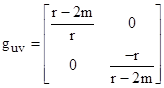 |
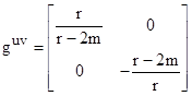
which has determinant g = -1. The inverse of the covariant tensor guv is the contravariant tensor
|
 |
To make use of index notation we define x1 = t and x2 = r, and then the equations for the geodesic paths in this manifold can be expressed as
|
 |
where summation is implied over any indices that are repeated in a given product, and Gijk denotes the Christoffel symbols. Note that the index i can be either 1 or 2, so the above expression actually represents two differential equations involving the 1st and 2nd derivatives of our coordinates x1 and x2 (which, remember, are just t and r) with respect to the proper time t for timelike paths.
|
The Christoffel symbol is defined in terms of the partial derivatives of the components of the metric tensor as follows
|
 |
Taking the partials of the components of our guv with respect to t and r we find that they are all zero, with the exception of
|
 |
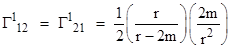
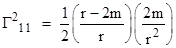
Combining this with the fact that the only non-zero components of the inverse metric tensor guv are g11 and g22, we find that the only non-zero Christoffel symbols are
|
 |
 |
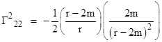 |
So, substituting these expressions into the geodesic formula (2), and reverting back to the symbols t and r for our coordinates, we have the two ordinary differential equations for the geodesic paths on the surface
|
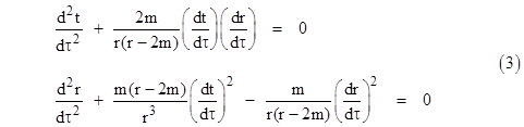 |
These equations can be integrated in closed form (see below), but they can also be directly integrated numerically using small incremental steps of dτ. For any given initial position and trajectory we can generate the subsequent geodesic path in terms of r as a function of t. We find that such paths invariably go to infinite t as r approaches 2m. Is our two-dimensional surface actually singular at r = 2m, or are the coordinates simply ill-behaved (like longitude at the North pole)?
|
As we saw above, the surface has an invariant Gaussian curvature at each point. Let's determine the curvature to see if anything strange occurs at r = 2m. The curvature can be computed in terms of the components of the metric tensor and their first and second partial derivatives. The non-zero first derivatives for our surface (and the determinant g = -1) were noted above. The only non-zero second derivatives are
|
 |
So we can compute the intrinsic curvature of our surface using Gauss's formula for the curvature invariant K of a two-dimensional surface given in Section 5.3. Inserting the metric components and derivatives for our surface into that equation gives the intrinsic curvature
|
 |
Therefore, at r = 2m the curvature of this surface is -1/(4m2), which is certainly finite, and in fact can be made arbitrarily small for sufficiently large m. The only singularity in the intrinsic curvature of the surface occurs at r = 0.
|
In order to solve the geodesic equations (3) for r as a function of the proper time t we first re-write the second geodesic equation in the form
|
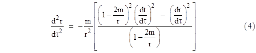 |
Since the basic line element (1) implies
|
 |
it follows that the quantity in the square brackets in (4) is unity, so we have
|
 |
Furthermore, notice that the derivative with respect to τ of the expression on the right hand side equation (5) is
|
 |
where we’ve made use of equation (6). Therefore, the expression in the square brackets on the left side is a constant (corresponding to the constant sum of potential plus kinetic energy), whose value for any given trajectory can be determined at any convenient point. For a bounded trajectory there is a radial position R, the apogee of the path, where dr/dτ = 0, and hence for any such trajectory we have
|
 |
On the other hand, for an unbounded trajectory there is no apogee, but instead the velocity dr/dt approaches an asymptotic value V as r goes to infinity. Noting that dr/dτ = (dr/dt)(dt/dτ) and making use of the basic line element (1) to give dt/dτ in terms of dr/dt, we have
|
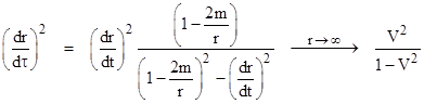 |
Therefore, for an unbounded radial trajectory with asymptotic speed V we have
|
 |
As an aside, we note that although we’ve asserted that the quantity in square brackets on the right side of equation (4) is unity, the denominator is zero at r = 2m, so the expression is actually singular at that point. However, it is a removable singularity, because the numerator also goes to zero at r = 2m, canceling the zero in the denominator. This implies that (dr/dt)2 is invariably forced to 1 - 2m/R precisely at r = 2m for bounded trajectories, and to 1/(1−V2) for unbounded trajectories.
|
Focusing on bounded trajectories, we return to (7a) and note that it implies
|
 |
Taking the square root and re-arranging terms, this gives
|
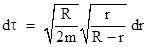 |
We have the integral
|
 |
To simplify this result, we make a change of variables by defining the argument of the inverse sine to be the cosine of some angle a. Thus we define a such that cos(a) = 2r/R – 1, which implies
|
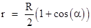 |
Inserting this into the preceding equation gives the elapsed proper time between r1 = R and r2 = r as
|
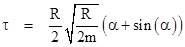 |
This shows that equation (6) has the same closed-form solution as does radial free-fall in Newtonian mechanics (as shown in Section 4.3 if t is identified with Newton's coordinate time t), namely, the parametric "cycloid relations". A plot of this r versus t corresponds to the position of a point on the rim of a rolling wheel of radius R/2, where a is the angle of the wheel.
|
We can also express the Schwarzschild coordinate time t explicitly in terms of a by multiplying the two relations
|
 |
to give
|
 |
Substituting the parametric expression for r into this equation, multiplying through by da, and integrating both sides, we get
|
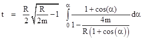 |
The integral can be evaluated explicitly to give
|
 |
Now, making use of the trigonometric identity
|
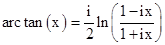 |
the equation can be written in the form
|
 |
where Q =
 . For values of a corresponding to r < 2m the argument of the logarithm is negative, and hence the value of the logarithm is offset by pi. This occurs because, in such cases, we are integrating from a = 0 where r = R (which is greater than 2m) to a value of a corresponding to r less than 2m, and hence we must perform a complex integration around the singularity at r = 2m, offsetting the result by ±pi (assuming the path of integration doesn’t make any complete loops around the singularity). This is not surprising, because the t coordinates are discontinuous at r = 2m, so we cannot unambiguously “carry over” the labeling of the t coordinates in the region r > 2m to the region r < 2m. In general, since the metric coefficients are independent of t, the t labels for events outside r = 2m can all be offset by a constant value without affecting any of our results, and likewise the t labels for events inside r = 2m can all be offset by a constant value. Moreover, the t label offsets for the inner and outer regions are independent of each other, because of the discontinuity at r = 2m. Lacking any definite interior boundary condition, we are free to choose the interior offset such that t is real-valued. The real part of ln(z) for any complex z, positive or negative, is ln(|z|), so we can simply stipulate that we will take the absolute value of the argument of the logarithm, i.e., we define the t coordinates by . For values of a corresponding to r < 2m the argument of the logarithm is negative, and hence the value of the logarithm is offset by pi. This occurs because, in such cases, we are integrating from a = 0 where r = R (which is greater than 2m) to a value of a corresponding to r less than 2m, and hence we must perform a complex integration around the singularity at r = 2m, offsetting the result by ±pi (assuming the path of integration doesn’t make any complete loops around the singularity). This is not surprising, because the t coordinates are discontinuous at r = 2m, so we cannot unambiguously “carry over” the labeling of the t coordinates in the region r > 2m to the region r < 2m. In general, since the metric coefficients are independent of t, the t labels for events outside r = 2m can all be offset by a constant value without affecting any of our results, and likewise the t labels for events inside r = 2m can all be offset by a constant value. Moreover, the t label offsets for the inner and outer regions are independent of each other, because of the discontinuity at r = 2m. Lacking any definite interior boundary condition, we are free to choose the interior offset such that t is real-valued. The real part of ln(z) for any complex z, positive or negative, is ln(|z|), so we can simply stipulate that we will take the absolute value of the argument of the logarithm, i.e., we define the t coordinates by |
 |
This gives a purely real-valued labeling of the t coordinates that satisfies the condition on the derivative at every point (except of course where the t coordinates are singular at r = 2m). Strictly speaking, we could further offset the interior labels by any real constant, so the above expression for the coordinate time of a free-falling particle is not unique, but it is the simplest matching of the t labels. On this basis, a typical timelike radial orbit is illustrated below, both in terms of proper time and Schwarzschild coordinate time, as function of the parameter a.
|
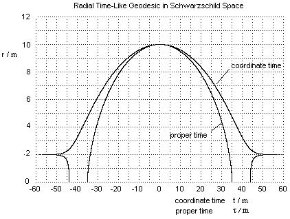 |
A notable feature of this trajectory is its temporal symmetry. Not only is there a continuous geodesic path from the apogee down through the Schwarzschild radius to the singularity at r = 0, there is also a continuous geodesic path from the singularity up through the Schwarzschild radius to the apogee. This was to be expected in view of the temporal symmetry of the field equations in general, and the Schwarzschild metric in particular, but it might seem inconsistent with the well-known fact that once a particle has crossed from outside to inside the Schwarzschild radius it can never re-emerge. However, there is no inconsistency, because the emerging particle has never crossed from outside to inside that radius.
|
To understand the full set of possible trajectories consistent with the Schwarzschild metric, it’s useful to first note an ambiguity present in all pseudo-Riemannian metrics due to their quadratic character. Consider the Minkowski metric (dt)2 = (dt)2 – (dx)2, which obviously doesn’t constrain the signs of the differentials, because they each appear squared. At constant x this metric requires (dt/dt)2 = 1, but the ratio dt/dt itself can be either +1 or −1. Strictly speaking, we are free to choose whether the proper time along a given path increases or decreases as the coordinate time increases. We might fancifully imagine that the Minkowski metric actually entails two separate universes, with proper time increasing with coordinate time in one, and decreasing with coordinate in the other. Alternatively we could imagine a single universe with two families of particles, whose proper times increase in opposite directions of the coordinate time t. (In fact, John Wheeler once speculated that anti-matter particles might be modeled as particles moving backward in time.) However, with a fixed metric like the Minkowski metric, it’s easy to just arbitrarily stipulate the same sign for dt and dt for every path, and then continuity requires that this always remains true (since timelike paths cannot “turn around” in Minkowski space).
|
The same quadratic ambiguity arises when considering the Schwarzschild metric, but in this case the various possible signs of the differentials are more inter-related, because the coefficients of the metric change signs at r = 2m. For values of r greater than 2m we have a metric of the form (dt)2 = (dt)2 – (dr)2 neglecting scale factors, whereas for values of r less than 2m the metric takes the form (dt)2 = (dr)2 – (dt)2. In the former case, |dt| must always equal or exceed |dt|, but in the latter case |dr| must equal or exceed |dt|. Thus, outside the Schwarzschild radius we must choose the sign of dt/dt, and inside that radius we must choose the sign of dr/dt. The signs of these ratios cannot change along any particle’s path in their respective regions. In effect, the radius r serves as the “time” coordinate inside the Schwarzschild radius.
|
Now, by analytic continuation, it can be shown that a path crossing the Schwarzschild radius from an outer region must enter an inner region with negative dr/dt. This is why a particle falling inward through the Schwarzschild radius must thereafter continue to reach smaller and smaller values of r. It cannot “turn around”, but must continue down to r = 0. However, conversely, it can be shown that a particle passing outward through the Schwarzschild radius must have come from an inner region of positive dr/dt. Hence if we observe objects falling into the inner region, and other objects emerging from the inner region, we seem forced to conclude that there are two physically distinct inner regions, or else that there exist closed spacetime loops if we insist on a single interior region. One or the other of these consequences is unavoidable if we take seriously the analytic continuation of all geodesics consistent with the Schwarzschild metric. The existence of two distinct inner regions is perhaps not surprising if we note that an in-falling object requires infinite coordinate time to cross the boundary at r = 2m, and conversely an out-going object requires infinite coordinate time to emerge. Clearly these are two very different classes of objects, one coming from the beginning of coordinate time, and the other departing to the end of coordinate time. The same reasoning leads to the potential existence of a second outer region, with negative dt/dt, so the full extent of the manifold entailed by the Schwarzschild metric, if fully developed, consists of four distinct regions. Thus the consideration of simple radial trajectories in Schwarzschild spacetime leads unavoidably to cosmological issues, which are described more fully in the discussions of “black holes” in Section 7.
|
In the preceding discussion we have focused on time-like radial paths, taking the proper time τ as the path length parameter. As noted in Section 6.1, for light-like paths we have dτ = 0 and so the metric (1) reduces to simply (1 – 2m/r)2(dt)2 = (dr)2, and thus we have, for any r2 and r1 greater than 2m, the coordinate time difference
|
 |
As expected, if m = 0 this reduces to (t2 – t1) = ±(r2 – r1). For non-zero m, we see that dr/dt = 0 at r = 2m (where these coordinates are ill-conditioned), and it isn’t obvious from this expression how to extrapolate through that boundary.
|
One way of clarifying all possible radial paths, time-like and light-like, consistent with the Schwarzschild solution is to re-write the radial line element (1) as
|
 |
If we define a new radial coordinate r so that the second term in the square brackets is (dr)2, then light rays will be diagonal lines when plotted in terms of t and r. Thus we set
|
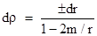 |
Notice that either sign is possible, since only the squared differential appears in (9). Integrating both sides and choosing a suitable constant of integration, we define r explicitly by
|
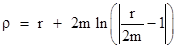 |
The absolute value is used to reverse the signs at r = 2m, so that the argument of the logarithm is always non-negative. (Note that the derivative of r with respect to r is invariant under reversal of sign of the argument of the logarithm.) This relation can also be written in the form
|
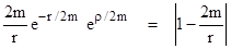 |
so we can write the radial Schwarzschild line element (9) in the form
|
 |
where r is now regarded as a function of r. The leading coefficient on the right side is well-behaved except at r = 0, but the trailing coefficient is singular at r = 2m, where r is infinite. Since dt is finite at that point, we infer that (dt)2 – (dr)2 must be identically zero at that point. We wish to absorb the trailing coefficient into the differentials to give an explicitly finite expression for (dt)2. Notice that in terms of coordinates A and B defined such that r = A+B and t = A-B the line element has the form
|
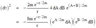 |
Recalling that d(ex) = exdx, we see that we can absorb the exponential coefficients into the differentials by simply defining the coordinates
|
 |
The line element in terms of these coordinates has the simple form
|
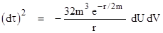 |
For convenience we can now return to the orthogonal hyperbolic form by making one more change of coordinates, defining u and v such that U = u+v and V = u-v. Making these substitutions, we get
|
 |
where, as noted previously, the parameter r is treated as a function of u and v. These are called Kruskal-Szekeres coordinates. Making all the substitutions for the changes of variables, we see that they are given explicitly as functions of r and t by
|
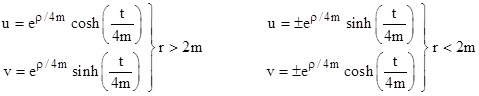 |
The signs for the case r < 2m are positive in the collapsing interior region and negative in the expanding interior region. A plot of the Schwarzschild solution in terms of these coordinates is shown below.
|
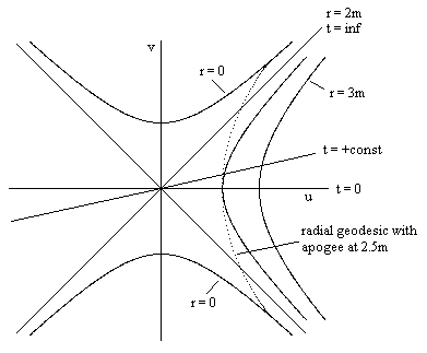 |
The dotted curve represents a complete time-like radial geodesic. As discussed previously, this curve is temporally symmetrical, emerging from the r = 0 singularity, rising through the r = 2m horizon to the apogee (which is at 2.5m in this plot), and then falling back through the r = 2m horizon to the singularity at r = 0. These coordinates confirm that there are actually two singularities in this fully developed solution. The lower r = 0 locus in the plot is the singularity at the center of a “white hole”, and r is always increasing with proper time in the region surrounding this singularity. The upper r = 0 locus is the singularity at the center of a “black hole”, and r is always decreasing with proper time in the region surrounding this singularity. The spatial region to the right of the v axis is our usual external universe, whereas the mirror region on the left is a separate universe. However, the physical applicability of this analytically complete solution is highly dubious, because no known physical process would lead to such a result. The “black holes” to be discussed in Section 7, hypothesized to result from the gravitational collapse of stars, do not entail this complete solution, so the global topology of the complete Schwarzschild solution, as exhibited by the Kruskal coordinates, is presumably of only theoretical interest.
|


grand design.. – Vineet Menon Apr 10 '12 at 15:27