工程电磁场 - 第 19 頁 - Google 圖書結果
books.google.com.hk/books?isbn=7302091617 - 轉為繁體網頁
将所有面积元的这些线积分相加,可以看出,因为在各个小回路公共边界上的积分路径
[PDF]
工程电磁场 - 数字图书馆
book.heze.cc/date%5CO%5CA2088431.pdf
路公共边界上的积分路径方向彼此相反,使得这部分积分互. 相抵消,只有外边界的那部分积分存在。所以,积分的结果. 是所有沿小回路积分的总和等于沿大回路l 的 ...
工程电磁场 - 第 19 頁 - Google 圖書結果
books.google.com.hk/books?isbn=7302091617 - 轉為繁體網頁
将所有面积元的这些线积分相加,可以看出,因为在各个小回路公共边界上的积分路径Math Insight
The idea behind Stokes' theorem
Stokes' theorem is a generalization of Green's theorem from circulation in a planar region to circulation along a surface. Green's theorem states that, given a continuously differentiable two-dimensional vector field F
, the integral of the “microscopic circulation” of F
over the region D
inside a simple closed curve C
is equal to the total circulation of F
around C
, as suggested by the equation
∫CF⋅ds=∬D“microscopic circulation of F” dA.
We often write that C=∂D
as fancy notation meaning simply that C
is the boundary of D
. Green's theorem requires that C=∂D
.
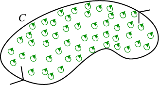
The “microscopic circulation” in Green's theorem is captured by the curl of the vector field and is illustrated by the green circles in the below figure.
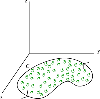
Green's theorem applies only to two-dimensional vector fields and to regions in the two-dimensional plane. Stokes' theorem generalizes Green's theorem to three dimensions. For starters, let's take our above picture and simply embed it in three dimensions. Then, our curveC
becomes a curve in the xy
-plane, and our region D
becomes a surface S
in the xy
-plane whose boundary is the curve C
. Even though S
is now a surface, we still use the same notation as ∂
for the boundary. The boundary ∂S
of the surface S
is a closed curve, and we require that ∂S=C
.
The next question is what the microscopic circulation along a surface should be. For Green's theorem, we found that
“microscopic circulation”=(curlF)⋅k,
(where k
is the unit-vector in the z
-direction). We wanted the component of the curl in the k
direction because this corresponded to microscopic circulation in the xy
-plane. Similarly, for a surface, we will want the microscopic circulation along the surace. This corresponds to the component of the curl that is perpendicular to the surface, i.e,
“microscopic circulation”=(curlF)⋅n,
where n
is a unit normal vector to the surface. You can see this using the right-hand rule. If you point the thumb of your right hand perpendicular to a surface, your fingers will curl in a direction corresponding to circulation parallel to the surface.
In summary, to go from Green's theorem to Stoke's theorem, we've made two changes. First, we've changed the line integral living in two dimensions (Green's theorem) to a line integral living in three dimensions (Stokes' theorem). Second, we changed the double integral ofcurlF⋅k
over a region D
in the plane (Green's theorem) to a surface integral of curlF⋅n
over a surface floating in space (Stokes' theorem). The required relationship between the curve C
and the surface S
(Stokes' theorem) is identical to the relationship between the curve C
and the region D
(Green's theorem): the curve C
must be the boundary ∂D
of the region or the boundary ∂S
of the surface.
We write Stokes' theorem as:
∫CF⋅ds=∬ScurlF⋅ndS=∬ScurlF⋅dS
(Recall that a surface integral of a vector field is the integral of the component of the vector field perpendicular to the surface.) We see that the integral on the right is the surface integral of the vector field curlF
. Stokes theorem says the surface integral of curlF
over a surface S
(i.e., ∬ScurlF⋅dS
) is the circulation of F
around the boundary of the surface (i.e., ∫CF⋅ds
where C=∂S
).
Once we have Stokes' theorem, we can see that the surface integral ofcurlF
is a special integral. The integral cannot change if we can change the surface S
to any surface as long as the boundary of S
is still the curve C
. It cannot change because it still must be equal to ∫CF⋅ds
, which doesn't change if we don't change C
. (In analogy of how the gradient ∇f
is a path-independent vector field, you could say that curlF
is “surface independent” vector field, but we don't usually use that term.)
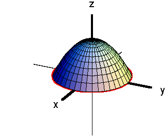
For example, staring with a planar surface such as sketched above, we see that the surfaceS
doesn't have to be the flat surface inside C
. We can bend and stretch S
, and the above formula is still true. In the below applet, you can move the blue point on the slider to change the surface S
. For any of those surfaces, the integral of the “microscopic circulation” curlF
over that surface will be the total circulation ∫CF⋅ds
of F
around the curve C
(shown in red). The important restriction is that the boundary of the surface S
is still the curve C
.
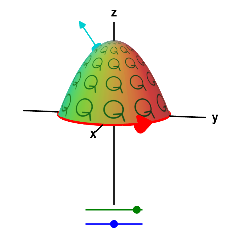 Macroscopic and microscopic circulation in three dimensions. The relationship between the macroscopic circulation of a vector field
 F
around a curve and the microscopic circulation of F
(illustrated by small green circles) along a surface in three dimensions must hold for any surface whose boundary is the curve. No matter which surface you choose (change by dragging the blue point on the slider), the total microscopic circulation of F
along the surface must equal the circulation of F
around the curve, as long as the vector field F
is defined everywhere on the surface.
More information about applet. Stokes' theorem allows us to do even more. We don't have to leave the curve C
sitting in the xy
-plane. We can twist and turn C
as well. If S
is a surface whose boundary is C
(i.e., if C=∂S
), it is still true that
∫CF⋅ds=∬ScurlF⋅dS.
For example, in the below applet, you can move the blue point on the slider to change the surface S
, as before. But, you can also move the green point on the slider to change the curve C
. The surface S
also changes as you change C
, since its boundary has to be C
. (Although the applet doesn't show the green circles representing the “microscopic circulation,” you can imagine what they would look like.)
 Changing surfaces in Stokes' theorem. Since Stokes' theorem states that the integral of the microscopic circulation
 curlF
over a surface is equal to the circulation of F
around the surface boundary (in red), changing the surface without changing the boundary (by dragging blue point on the slider) cannot change the surface integral of curlF
. On the other hand, if you change the boundary (by dragging the green point on the slider), then both the surface integral and the line integral defining the circulation around the boundary do change, though they are still equal to each other.
More information about applet. Note that moving the blue dot on the slider does not change the value of either integral in the above formulas. Since the curve C
does not change, the left line integral doesn't change, which means the value of the right surface integral cannot change. On the other hand, moving the green dot on the slider does change the values of the integrals since the curve C
changes. The important point is that, even in this case, the left line integral and the right surface integral are always equal.
There is one more subtlety that you have to get correct, or else you'll may be off by a sign. You need to orient the surface and boundary properly.
You can read some examples here.
The “microscopic circulation” in Green's theorem is captured by the curl of the vector field and is illustrated by the green circles in the below figure.
Green's theorem applies only to two-dimensional vector fields and to regions in the two-dimensional plane. Stokes' theorem generalizes Green's theorem to three dimensions. For starters, let's take our above picture and simply embed it in three dimensions. Then, our curve
The next question is what the microscopic circulation along a surface should be. For Green's theorem, we found that
In summary, to go from Green's theorem to Stoke's theorem, we've made two changes. First, we've changed the line integral living in two dimensions (Green's theorem) to a line integral living in three dimensions (Stokes' theorem). Second, we changed the double integral of
We write Stokes' theorem as:
Once we have Stokes' theorem, we can see that the surface integral of
For example, staring with a planar surface such as sketched above, we see that the surface
More information about applet.
More information about applet.
There is one more subtlety that you have to get correct, or else you'll may be off by a sign. You need to orient the surface and boundary properly.
You can read some examples here.
Thread navigation
Math 2374
Multivariable calculus
Notation systems
More information on notation systemsSimilar pages
- Proper orientation for Stokes' theorem
- The idea behind Green's theorem
- Stokes' theorem examples
- The definition of curl from line integrals
- Calculating the formula for circulation per unit area
- The integrals of multivariable calculus
- The components of the curl
- Subtleties about curl
- The idea of the curl of a vector field
- A path-dependent vector field with zero curl
- More similar pages
No comments:
Post a Comment