In linear regression y is Gaussian; in logistic regression y is Bernoulli. beta with a hat , Binomial regression models are essentially the same as binary choice models, one type of discrete choice model. The primary difference is in the theoretical motivation: Discrete choice models are motivated using utility theory so as to handle various types of correlated and uncorrelated choices, while binomial regression models are generally described in terms of the generalized linear model, an attempt to generalize various types of linear regression models.

https://www.cs.princeton.edu/courses/archive/fall11/cos597C/lectures/hierarchical-models.pdf

• Regression is a field. There are sequences of classes taught about it. • Notation and terminology – Response variable yi is what we try to predict. – Predictor vector xi are attributes of the ith data point. – Coefficients β are regression parameters. • The two regression models everyone has heard of are – Linear regression for continuous responses, yi | xi ∼ N (β > xi ,σ 2 ) (6) – Logistic regression for binary responses (e.g., spam classification), p(yi = 1| xi) = logit(β > xi) (7) – In both cases, the distribution of the response is governed by the linear combination of coefficients (top level) and predictors (specific for the ith data point). • We can use regression for prediction. – The coefficient component βi tells us how the expected value of the response changes as a function of each attribute. – For example, how does the literacy rate change as a function of the dollars spent on library books? Or, as a function of the teacher/student ratio? – How does the probability of my liking a song change based on its tempo? • We can also use regression for description. 7 – Given a new song, what is the expected probability that I will like it? – Given a new school, what is the expected literacy rate? • Linear and logistic regression are examples of generalized linear models. – The response yi is drawn from an exponential family, p(yi | xi) = exp{η(β, xi) > t(yi)− a(η(β, xi))}. (8) – The natural parameter is a function η(β, xi) = f (β >xi). – In many cases, η(β, xi) = β >xi . • Discussion – In linear regression y is Gaussian; in logistic regression y is Bernoulli. – GLMs can accommodate discrete/continuous, univariate/multivariate responses. – GLMs can accommodate arbitrary attributes. – (Recall the discussion of sparsity and GLMs in COS513.) • Nelder and McCallaugh is an excellent reference about GLMs. (Nelder invented them.)

http://www.theanalysisfactor.com/confusing-statistical-term-4-hierarchical-regression-vs-hierarchical-model/

Andy December 18, 2009 at 8:10 am

I find SPSS’s use of beta for standardised coefficients tremendously annoying!

BTW a beta with a hat on is sometimes used to denote the sample estimate of the population parameter. But mathematicians tend to use any greek letters they feel like using! The trick for maintaining sanity is always to introduce what symbols denote.

REPLY

 Karen December 21, 2009 at 5:38 pm

Ah, yes! Beta hats. This is actually “standard” statistical notation. The sample estimate of any population parameter puts a hat on the parameter. So if beta is the parameter, beta hat is the estimate of that parameter value.

What are type I and type II errors?

Learn more about Minitab 17 

When you do a hypothesis test, two types of errors are possible: type I and type II. The risks of these two errors are inversely related and determined by the level of significance and the power for the test. Therefore, you should determine which error has more severe consequences for your situation before you define their risks.

No hypothesis test is 100% certain. Because the test is based on probabilities, there is always a chance of drawing an incorrect conclusion.

Type I error

When the null hypothesis is true and you reject it, you make a type I error. The probability of making a type I error is α, which is the level of significance you set for your hypothesis test. An α of 0.05 indicates that you are willing to accept a 5% chance that you are wrong when you reject the null hypothesis. To lower this risk, you must use a lower value for α. However, using a lower value for alpha means that you will be less likely to detect a true difference if one really exists.

Type II error

When the null hypothesis is false and you fail to reject it, you make a type II error. The probability of making a type II error is β, which depends on the power of the test. You can decrease your risk of committing a type II error by ensuring your test has enough power. You can do this by ensuring your sample size is large enough to detect a practical difference when one truly exists.

The probability of rejecting the null hypothesis when it is false is equal to 1–β. This value is the power of the test.

	Null Hypothesis
Decision	True	False
Fail to reject	Correct Decision (probability = 1 - α)	Type II Error - fail to reject the null when it is false (probability = β)
Reject	Type I Error - rejecting the null when it is true (probability = α)	Correct Decision (probability = 1 - β)

Example of type I and type II error

To understand the interrelationship between type I and type II error, and to determine which error has more severe consequences for your situation, consider the following example.

A medical researcher wants to compare the effectiveness of two medications. The null and alternative hypotheses are:

• Null hypothesis (H0): μ1= μ2
  The two medications are equally effective.
• Alternative hypothesis (H1): μ1≠ μ2
  The two medications are not equally effective.

A type I error occurs if the researcher rejects the null hypothesis and concludes that the two medications are different when, in fact, they are not. If the medications have the same effectiveness, the researcher may not consider this error too severe because the patients still benefit from the same level of effectiveness regardless of which medicine they take. However, if a type II error occurs, the researcher fails to reject the null hypothesis when it should be rejected. That is, the researcher concludes that the medications are the same when, in fact, they are different. This error is potentially life-threatening if the less-effective medication is sold to the public instead of the more effective one.

As you conduct your hypothesis tests, consider the risks of making type I and type II errors. If the consequences of making one type of error are more severe or costly than making the other type of error, then choose a level of significance and a power for the test that will reflect the relative severity of those consequences.

Binomial regression

From Wikipedia, the free encyclopedia

In statistics, binomial regression is a technique in which the response (often referred to as Y) is the result of a series of Bernoulli trials, or a series of one of two possible disjoint outcomes (traditionally denoted "success" or 1, and "failure" or 0).^[1] In binomial regression, the probability of a success is related to explanatory variables: the corresponding concept in ordinary regression is to relate the mean value of the unobserved response to explanatory variables.

Binomial regression models are essentially the same as binary choice models, one type of discrete choice model. The primary difference is in the theoretical motivation: Discrete choice models are motivated using utility theory so as to handle various types of correlated and uncorrelated choices, while binomial regression models are generally described in terms of the generalized linear model, an attempt to generalize various types of linear regression models. As a result, discrete choice models are usually described primarily with a latent variable indicating the "utility" of making a choice, and with randomness introduced through an error variable distributed according to a specific probability distribution. Note that the latent variable itself is not observed, only the actual choice, which is assumed to have been made if the net utility was greater than 0. Binary regression models, however, dispense with both the latent and error variable and assume that the choice itself is a random variable, with a link function that transforms the expected value of the choice variable into a value that is then predicted by the linear predictor. It can be shown that the two are equivalent, at least in the case of binary choice models: the link function corresponds to the quantile function of the distribution of the error variable, and the inverse link function to the cumulative distribution function (CDF) of the error variable. The latent variable has an equivalent if one imagines generating a uniformly distributed number between 0 and 1, subtracting from it the mean (in the form of the linear predictor transformed by the inverse link function), and inverting the sign. One then has a number whose probability of being greater than 0 is the same as the probability of success in the choice variable, and can be thought of as a latent variable indicating whether a 0 or 1 was chosen.

In machine learning, binomial regression is considered a special case of probabilistic classification, and thus a generalization of binary classification.

Contents

  [hide] 

• 1Example application
• 2Specification of model
• 3Link functions
• 4Comparison between binomial regression and binary choice models
• 5Latent variable interpretation / derivation
• 6See also
• 7Notes
• 8References

Example application[edit]

In one published example of an application of binomial regression,^[2] the details were as follows. The observed outcome variable was whether or not a fault occurred in an industrial process. There were two explanatory variables: the first was a simple two-case factor representing whether or not a modified version of the process was used and the second was an ordinary quantitative variable measuring the purity of the material being supplied for the process.

Specification of model[edit]

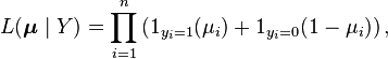
The results are assumed to be binomially distributed.^[1] They are often fitted as a generalised linear model where the predicted values μ are the probabilities that any individual event will result in a success. The likelihood of the predictions is then given by

where 1_A is the indicator function which takes on the value one when the event A occurs, and zero otherwise: in this formulation, for any given observation y_i, only one of the two terms inside the product contributes, according to whether y_i=0 or 1. The likelihood function is more fully specified by defining the formal parametersμ_i as parameterised functions of the explanatory variables: this defines the likelihood in terms of a much reduced number of parameters. Fitting of the model is usually achieved by employing the method of maximum likelihood to determine these parameters. In practice, the use of a formulation as a generalised linear model allows advantage to be taken of certain algorithmic ideas which are applicable across the whole class of more general models but which do not apply to all maximum likelihood problems.

Models used in binomial regression can often be extended to multinomial data.

There are many methods of generating the values of μ in systematic ways that allow for interpretation of the model; they are discussed below.

Link functions[edit]

There is a requirement that the modelling linking the probabilities μ to the explanatory variables should be of a form which only produces values in the range 0 to 1. Many models can be fitted into the form

Here η is an intermediate variable representing a linear combination, containing the regression parameters, of the explanatory variables. The function g is thecumulative distribution function (cdf) of some probability distribution. Usually this probability distribution has a range from minus infinity to plus infinity so that any finite value of η is transformed by the function g to a value inside the range 0 to 1.

In the case of logistic regression, the link function is the log of the odds ratio or logistic function. In the case of probit, the link is the cdf of the normal distribution. The linear probability model is not a proper binomial regression specification because predictions need not be in the range of zero to one; it is sometimes used for this type of data when the probability space is where interpretation occurs or when the analyst lacks sufficient sophistication to fit or calculate approximate linearizations of probabilities for interpretation.

Comparison between binomial regression and binary choice models[edit]

A binary choice model assumes a latent variable U_n, the utility (or net benefit) that person n obtains from taking an action (as opposed to not taking the action). The utility the person obtains from taking the action depends on the characteristics of the person, some of which are observed by the researcher and some are not:

where  is a set of regression coefficients and  is a set of independent variables (also known as "features") describing person n, which may be either discrete "dummy variables" or regular continuous variables.  is a random variable specifying "noise" or "error" in the prediction, assumed to be distributed according to some distribution. Normally, if there is a mean or variance parameter in the distribution, it cannot be identified, so the parameters are set to convenient values — by convention usually mean 0, variance 1.

The person takes the action, y_n = 1, if U_n > 0. The unobserved term, ε_n, is assumed to have a logistic distribution.

The specification is written succinctly as:

• • U_n = βs_n + ε_n
  • 
  • ε ∼ logistic, standard normal, etc.

Let us write it slightly differently:

• • U_n = βs_n − e_n
  • 
  • e ∼ logistic, standard normal, etc.

Here we have made the substitution e_n = −ε_n. This changes a random variable into a slightly different one, defined over a negated domain. As it happens, the error distributions we usually consider (e.g. logistic distribution, standard normal distribution, standard Student's t-distribution, etc.) are symmetric about 0, and hence the distribution over e_n is identical to the distribution over ε_n.

Denote the cumulative distribution function (CDF) of  as  and the quantile function (inverse CDF) of  as 

Note that

Since  is a Bernoulli trial, where  we have

or equivalently

Note that this is exactly equivalent to the binomial regression model expressed in the formalism of the generalized linear model.

If  i.e. distributed as a standard normal distribution, then

which is exactly a probit model.

If  i.e. distributed as a standard logistic distribution with mean 0 and scale parameter 1, then the corresponding quantile function is the logit function, and

which is exactly a logit model.

Note that the two different formalisms — generalized linear models (GLM's) and discrete choice models — are equivalent in the case of simple binary choice models, but can be exteneded if differing ways:

• GLM's can easily handle arbitrarily distributed response variables (dependent variables), not just categorical variables or ordinal variables, which discrete choice models are limited to by their nature. GLM's are also not limited to link functions that are quantile functions of some distribution, unlike the use of an error variable, which must by assumption have a probability distribution.
• On the other hand, because discrete choice models are described as types of generative models, it is conceptually easier to extend them to complicated situations with multiple, possibly correlated, choices for each person, or other variations.

Latent variable interpretation / derivation[edit]

A latent variable model involving a binomial observed variable Y can be constructed such that Y is related to the latent variable Y* via

The latent variable Y* is then related to a set of regression variables X by the model

This results in a binomial regression model.

The variance of ϵ can not be identified and when it is not of interest is often assumed to be equal to one. If ϵ is normally distributed, then a probit is the appropriate model and if ϵ is log-Weibull distributed, then a logit is appropriate. If ϵ is uniformly distributed, then a linear probability model is appropriate.

Logistic regression - Wikipedia, the free encyclopedia

https://en.wikipedia.org/wiki/Logistic_regression

Wikipedia

In statistics, logistic regression, or logit regression, or logit model is a regressionmodel where ... Logistic regression can be seen as a special case of generalizedlinear ... is a Bernoulli distribution rather than a Gaussian distribution, because the .... The associated latent variable is y\prime = \beta_0 + \beta_1 x + \epsilon .

You visited this page on 4/25/16.

Generalized linear model - Wikipedia, the free encyclopedia

https://en.wikipedia.org/wiki/Generalized_linear_model

Wikipedia

In statistics, the generalized linear model (GLM) is a flexible generalization of ordinarylinear regression that allows for response variables that have error distribution models other than a normal distribution. The GLM generalizes linear regression by allowing the linear model to be .... where E(Y) is the expected value of Y; Xβ is the linear predictor, a linear ...

Binomial regression - Wikipedia, the free encyclopedia

https://en.wikipedia.org/wiki/Binomial_regression

Wikipedia

In statistics, binomial regression is a technique in which the response is the result of a series of .... The linear probability model is not a proper binomial regressionspecification ... is a Bernoulli trial, where \mathbb{E}[Y_n] = \Pr(Y_n = 1) ... The latent variable Y* is then related to a set of regression variables X by the model.

[PDF]Logistic Regression - CMU Statistics

www.stat.cmu.edu/~cshalizi/uADA/.../ch12.p...

Carnegie Mellon University

coming up with a model for the joint distribution of outputs Y and inputs X, which can be quite ... Without some constraints, estimating the “inhomogeneous Bernoulli” model by max- ... So logistic regression gives us a linear classifier. ..... is the case where response is Gaussian, with mean equal to the linear predictor, and.

[PDF]Review: Logistic regression, Gaussian naïve Bayes, linear ...

https://www.cs.cmu.edu/.../Recitation_3.pdf

Carnegie Mellon University

Feb 3, 2011 - Review: Logistic regression, Gaussian naïve. Bayes, linear regression, and their connections. Yi Zhang. 10-701, Machine ... Logistic regression: assumptions on P(Y|X): ◦ And thus: 4 ... P(X,Y) = P(Y)P(X|Y). ◦ Bernoulli on Y:.

[PDF]1 Logistic regression

www.cs.princeton.edu/courses/archive/.../0410b.pdf

Princeton University

Apr 10, 2008 - Problems of binary classification with linear regression (in which yn ∼ N(βT x, σ2)): (1) it will ... classification, yn is either zero or one; not drawn fromGaussian.) Model y as Bernoulli: ... µ(x) = logistic(βT x): maps R → (0,1).

binomial - Logistic Regression - Error Term and its ...

stats.stackexchange.com/.../logistic-regression-error-term-and-its-distribu...

Nov 20, 2014 - In linear regression observations are assumed to follow a Gaussian ... In logistic regression observations y ∈ { 0 , 1 } are assumed to .... There is no error term in the Bernoulli distribution, there's just an unknown probability.

[PDF]Generalized Linear Models (GLM)

www.wright.edu/~thaddeus.tarpey/ES714glm.pdf

Wright State University

May 29, 2012 - response variable y as a function of one or more predictor variables. ...linear regression, we have E[y|x] = β0 + β1x; that is, the conditional expectation .... In the simple logistic regression model, the probability of success p ..... is the conditional mean of the Bernoulli response Y given values of the regressor.

[PDF]Lecture 2

www.stat.rutgers.edu/~mxie/stat586/.../lecture2brief.p...

Rutgers University

by LR Model

response yi is said to follow a Logistic regression model, if ... The response yi follows a Bernoulli distribution yi ∼ Bernoulli(πi). • Similar as in the regular ... amount increase in h(E(y)) with a unit increase in the kth covariate xk, when the .... We can specify the Gaussian linear regression model in the same style as we used to ...

[PDF]Generalized Linear Models - Statistics - University of Michigan

dept.stat.lsa.umich.edu/~kshedden/Courses/Stat600/Notes/glm.pdf

Dec 2, 2015 - transform Y so that the linear model assumptions are approximately ... general. Logistic regression is used for binary outcome data, where Y = 0 or Y = 1. ...regression. Since the mean and variance of a Bernoulli trial are linked, the ....Gaussian linear model: The density of Y |X can be written log p(Yi |Xi ) ...