Modelling income, wealth, and expenditure data by use of Econophysics

Modelling income, wealth, and expenditure data by use of Econophysics  
by  
Elvis Oltean
Doctoral Thesis   
Submitted in partial fulfilment of the requirements
for the award of
Doctor of Philosophy of Loughborough University

Sigmoid function

From Wikipedia, the free encyclopedia

Jump to: navigation, search

This article needs additional citations for verification. Please help improve this article by adding citations to reliable sources. Unsourced material may be challenged and removed. (May 2008)

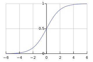
The logistic curve

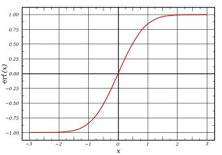
Plot of the error function

A sigmoid function is a mathematical function having an "S" shape (sigmoid curve). Often, sigmoid function refers to the special case of the logistic function shown in the first figure and defined by the formula

Other examples of similar shapes include the Gompertz curve (used in modeling systems that saturate at large values of t) and the ogee curve (used in the spillway of some dams). A wide variety of sigmoid functions have been used as the activation function of artificial neurons, including the logistic and hyperbolic tangent functions. Sigmoid curves are also common in statistics as cumulative distribution functions, such as the integrals of the logistic distribution, the normal distribution, and Student's t probability density functions.

Contents

 [hide] 

• 1 Definition
• 2 Properties
• 3 Examples
• 4 See also
• 5 References

Definition[edit]

A sigmoid function is a bounded differentiable real function that is defined for all real input values and has a positive derivative at each point.^[1]

CHAPTER 2:  APPLICATIONS OF LOGISTIC FUNCTIONTO THEDISTRIBUTION OF INCOME, WEALTH, AND EXPENDITURE 
Fermi-Dirac, Bose-Einstein, and Boltzmann-Gibbs distributions are the most important in statistical physics. Of these statistical physics distributions used so far for modelling socioeconomic systems with some degree of success were Bose-Einstein and Maxwell-Boltzmann distributions. The present chapter investigates the applications of logistic distribution to some of the most important economic variables such as income, wealth, and expenditure of the population from nine countries with different economic characteristics. This distribution was used outside economic systems initially and more recently it started being used due to the similarity of economic systems with biological and physical systems. 
2.1 Methodology 
The probability distribution used is cumulative logistic distribution which is applied to cumulated income, expenditure, or wealth on one hand and also to cumulated probabilities on the other hand. Logistic function or sigmoid function is defined as  
𝑓(𝑥) = 𝐿 1+𝑒𝑥𝑝−𝑘(𝑥−𝑥0)
 (2.1) 
where L is the curve's maximum value, x0 is the x-value of the sigmoid's midpoint, and k = the steepness of the curve[85]. Logistic map, which is the basis for logistic function, is used to show how complex, chaotic behaviour can arise from very simple non-linear dynamical equations [86]. 
We use logistic cumulative probability distribution C(x), which is defined as the integral 
C(x) = ∫ P(x)dx x −∞ (2.2)
23 
It gives the probability that a random variable is below a given value x. We present on y-axis the cumulated population probability, which is the share of population with income/wealth/expenditure lower than corresponding level on the x-axis. Cumulated income/wealth/expenditure is contained on the x-axis. According to this type of probability, we calculate the share of population having an income below a certain threshold. Thus, the probability to have an income lower than zero is 0 % (since everyone is assumed to have a certain income).
Cumulated income, wealth, or expenditure is contained on the x-axis. Let us assume X represents the values for cumulated income/wealth/expenditure represented on the x-axis. 
𝑋𝑖=∑𝑥𝑖 
where X represents the cumulated income/wealth/expenditure on the x-axis and  i=[1,10] for mean values and i=[1,9] for upper limit on income, where iєN. Thus, the decimal logarithm of probability, which is log10(C(x)), is the dependent probability and decimal logarithm of X (cumulated income) is the independent variable. Also, parameters a, b, and c are obtained from fitting the data using logistic distribution as described above in the eq. 2.2.
The results are produced using decimal logarithm values for both axes (i.e. log-log scale). Then, applying the log-log scale, the equation (2.1) becomes
𝑙𝑜𝑔10(𝐶(𝑋)) =
𝑎 1+𝑒𝑥𝑝𝑏(log10𝑋)+𝑐)
 (2.3) 
This is logarithmic form of logistic function. The total cumulated probability is 𝐶𝑖(𝑥 < 𝑋𝑖). In the case of mean income, the set which contains the plots representing the probability is S={ (0, 0%), (X1, 10%), (X2, 20%), (X3, 30%), (X4, 40%), (X5, 50%), (X6, 60%), (X7, 70%), (X8, 80%), (X9, 90%), (X10, 100%)}. In the case for the upper limit on income data sets, 𝑆1= {(0,0%), (X1, 10%), (X2, 20%), (X3, 30%), (X4, 40%), (X5, 50%), (X6, 60%), (X7, 70%), (X8, 80%), (X9, 90%). The fitting was made taking into account the decimal logarithmic values of the probability sets S and S1. The values for the tenth decile, which contains the upper income segment of population, is not comprised in the upper limit on income data set. For the lower limit on income, the set is similar except that each value represents the lowest expenditure value on income decile.  
24 
For the first decile (the lowest income decile), C represents the population that has an income lower than mean income or upper limit on income or lower limit of the first decile, hence equals 10%. For lower limit on income, the value for the first decile is 0. Subsequently, for the highest income the cumulative distribution function is 100 % (in case of mean income). For the upper limit on income and lower data sets, we do not represent the value for highest decile (tenth) because it was not made available by any of the statistical bodies.