phymath999: sas nonlinear programming code The objective function is the total free energy of the mixture.

http://mathworld.wolfram.com/BivariateNormalDistribution.html

http://blogs.sas.com/content/iml/2013/09/18/compute-a-contour-level-curve-in-sas.html

http://support.sas.com/documentation/cdl/en/imlug/59656/HTML/default/viewer.htm#nonlinearoptexpls_sect15.htm

Example 14.1 Chemical Equilibrium :: SAS/IML(R) 12.3 ...

support.sas.com/documentation/cdl/en/.../viewer.htm#...

SAS Institute

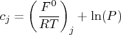
number of moles for compound $j$ , $j=1,\ldots ,n$. $s$. total number of moles in the mixture, $s=\sum _{i=1}^ n x_ j$. $a_{ij}$. number of atoms of element $i$ ...

The problem is to determine the parameters

that minimize the objective function

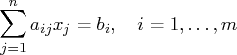
subject to the nonnegativity and linear balance constraints.

Moles of Compounds

The concept of a mole can be applied to compounds as well as elements. A mole of a compound is what you have when you weigh out, in grams, the formula weight of that compound. (Use the molecular weight if the compound is a molecular material.) For example, the formula weight for HF is 20.0. That means that one mole of HF weighs 20.0 grams, and you can use that relationship to convert back and forth between grams and moles.

For example, if you needed to change 15.0 g of HF to moles, you would simply multiply by the conversion factor that changes from gHF to moles HF. The relationship we just figured out is that 1 mole of HF weighs 20.0 g. Carrying out the calculations, we get 0.750 moles of HF.

15.0 g HF

x 1 mole HF
20.0 g HF

= 0.750 mole HF

To emphasize that this is the weight of one mole of that chemical, some chemists call it the molar formula weight or the mole weight or even the molar mass.

Top of Page

Back to Course Homepage

E-mail instructor: Sue Eggling
Clackamas Community College
©1998, 2002 Clackamas Community College, Hal Bender

2 Answers

Jing Conan Wang, Ph.D of Boston University Optimization, Machine Learning, Network Security

3.7k Views

In linear optimization, the boundary of feasible range is hyperplane and cost function is linear, too. If any of the constraints or the obj function is non-linear, the problem becomes non-linear optimization.

In optimization, there is a big difference between convex optimization and non-convex optimization, however, there is no intrinsic difference between linear programming and nonlinear programming.
Linear programming was studied first because it is easier to think in the pre-computer age. Simplex was popular mainly because it is easy to write down in paper (it is a tabular-based method). Note that complexity of Simplex is exponential.

Most of the polynomial-time algorithms (like interior point methods) work for both linear and non-linear programming.

Written 25 Feb 2015 • View Upvotes

Example 11.1: Chemical Equilibrium

The following example is used in many test libraries for nonlinear programming. It appeared originally in Bracken and McCormick (1968).

The problem is to determine the composition of a mixture of various chemicals that satisfy the mixture's chemical equilibrium state. The second law of thermodynamics implies that at a constant temperature and pressure, a mixture of chemicals satisfies its chemical equilibrium state when the free energy of the mixture is reduced to a minimum. Therefore, the composition of the chemicals satisfying its chemical equilibrium state can be found by minimizing the free energy of the mixture.

The following notation is used in this problem:

	number of chemical elements in the mixture
	number of compounds in the mixture
	number of moles for compound ,
	total number of moles in the mixture, $s=\sum_{i=1}^n x_j$
$a_{ij}$	number of atoms of element in a molecule of compound
	atomic weight of element in the mixture

The constraints for the mixture are as follows. Each of the compounds must have a nonnegative number of moles.

$x_j \geq 0 , j=1, ... ,n$

There is a mass balance relationship for each element. Each relation is given by a linear equality constraint.

$\sum_{j=1}^n a_{ij} x_j = b_i , i=1, ... ,m$

The objective function is the total free energy of the mixture.

$f(x) = \sum_{j=1}^n x_j [c_j + \ln ( {x_j \over s} ) ]$

where

$c_j = ( {f^0 \over rt} )_j + \ln(p)$

and

is the model standard free energy function for the

th compound. The value of

is found in existing tables.

is the total pressure in atmospheres.

The problem is to determine the parameters

that minimize the objective function

subject to the nonnegativity and linear balance constraints. To illustrate this, consider the following situation. Determine the equilibrium composition of compound $\frac{1}2 n_2 h_4 + \frac{1}2 o_2$ at temperature $t = 3500^{\circ} k$ and pressure

. The following table gives a summary of the information necessary to solve the problem.

				$a_{ij}$
				=1	=2	=3
	Compound			H	N	O
1		-10.021	-6.089	1
2		-21.096	-17.164	2
3		-37.986	-34.054	2		1
4		-9.846	-5.914		1
5		-28.653	-24.721		2
6		-18.918	-14.986	1	1
7		-28.032	-24.100		1	1
8		-14.640	-10.708			1
9		-30.594	-26.662			2
10		-26.111	-22.179	1		1

The following statements solve the minimization problem:

  
    proc iml; 
       c = { -6.089 -17.164 -34.054  -5.914 -24.721 
             -14.986 -24.100 -10.708 -26.662 -22.179 }; 
       start F_BRACK(x) global(c); 
          s = x[+]; 
          f = sum(x # (c + log(x / s))); 
          return(f); 
       finish F_BRACK; 
  
       con = { .  .  .  .  .  .  .  .  .  .    .   .  , 
               .  .  .  .  .  .  .  .  .  .    .   .  , 
               1. 2. 2. .  .  1. .  .  .  1.   0.  2. , 
               .  .  .  1. 2. 1. 1. .  .  .    0.  1. , 
               .  .  1. .  .  .  1. 1. 2. 1.   0.  1. }; 
       con[1,1:10] = 1.e-6; 
  
       x0 = j(1,10, .1); 
       optn = {0 3}; 
  
       title 'NLPTR subroutine: No Derivatives'; 
       call nlptr(xres,rc,"F_BRACK",x0,optn,con);

The F_BRACK module specifies the objective function,

. The matrix CON specifies the constraints. The first row gives the lower bound for each parameter, and to prevent the evaluation of the $\log(x)$ function for values of

that are too small, the lower bounds are set here to 1E-6. The following three rows contain the three linear equality constraints.

The starting point, which must be given to specify the number of parameters, is represented by X0. The first element of the OPTN vector specifies a minimization problem, and the second element specifies the amount of printed output.

The CALL NLPTR statement runs trust-region minimization. In this case, since no analytic derivatives are specified, the F_BRACK module is used to generate finite-difference approximations for the gradient vector and Hessian matrix.

The output is shown in the following figures. The iteration history does not show any problems.

Optimization Start
Active Constraints	3	Objective Function	-45.05516448
Max Abs Gradient Element	4.4710303342	Radius	1

Iteration	Restarts	Function Calls	Active Constraints		Objective Function	Objective Function Change	Max Abs Gradient Element	Lambda	Trust Region Radius
1	0	2	3	'	-47.33413	2.2790	4.3613	2.456	1.000
2	0	3	3	'	-47.70051	0.3664	7.0044	0.908	0.418
3	0	4	3		-47.73117	0.0307	5.3051	0	0.359
4	0	5	3		-47.73426	0.00310	3.7015	0	0.118
5	0	6	3		-47.73982	0.00555	2.3054	0	0.0169
6	0	7	3		-47.74846	0.00864	1.3029	90.184	0.00476
7	0	9	3		-47.75796	0.00950	0.5073	0	0.0134
8	0	10	3		-47.76094	0.00297	0.0988	0	0.0124
9	0	11	3		-47.76109	0.000155	0.00447	0	0.0111
10	0	12	3		-47.76109	3.385E-7	0.000011	0	0.00332

Optimization Results
Iterations	10	Function Calls	13
Hessian Calls	11	Active Constraints	3
Objective Function	-47.76109086	Max Abs Gradient Element	7.3901293E-6
Lambda	0	Actual Over Pred Change	0
Radius	0.0033214552

The output lists the optimal parameters with the gradient.

Optimization Results
Parameter Estimates
N	Parameter	Estimate	Gradient Objective Function
1	X1	0.040668	-9.785055
2	X2	0.147730	-19.570111
3	X3	0.783154	-34.792170
4	X4	0.001414	-12.968920
5	X5	0.485247	-25.937841
6	X6	0.000693	-22.753976
7	X7	0.027399	-28.190992
8	X8	0.017947	-15.222060
9	X9	0.037314	-30.444119
10	X10	0.096871	-25.007115

Value of Objective Function = -47.76109086

The three equality constraints are satisfied at the solution.

Linear Constraints Evaluated at Solution
1	ACT	-3.053E-16	=	-2.0000	+	1.0000	*	X1	+	2.0000	*	X2	+	2.0000	*	X3	+	1.0000	*	X6	+	1.0000	*	X10
2	ACT	-1.735E-17	=	-1.0000	+	1.0000	*	X4	+	2.0000	*	X5	+	1.0000	*	X6	+	1.0000	*	X7
3	ACT	-1.527E-16	=	-1.0000	+	1.0000	*	X3	+	1.0000	*	X7	+	1.0000	*	X8	+	2.0000	*	X9	+	1.0000	*	X10

The Lagrange multipliers and the projected gradient are also printed. The elements of the projected gradient must be small to satisfy a first-order optimality condition.

First Order Lagrange Multipliers
Active Constraint		Lagrange Multiplier
Linear EC	[1]	-9.785055
Linear EC	[2]	-12.968922
Linear EC	[3]	-15.222061

Projected Gradient
Free Dimension	Projected Gradient
1	0.000000328
2	-9.703359E-8
3	3.2183113E-8
4	-0.000007390
5	-0.000005172
6	-0.000005669
7	-0.000000937

phymath999

Wednesday, March 30, 2016

sas nonlinear programming code The objective function is the total free energy of the mixture.

http://mathworld.wolfram.com/BivariateNormalDistribution.html

Example 14.1 Chemical Equilibrium :: SAS/IML(R) 12.3 ...

Moles of Compounds

What is the difference between linear and non-linear optimization?

Related Questions

Example 11.1: Chemical Equilibrium

No comments:

Post a Comment