§1.6 电子和磁性对热膨胀的贡献_CNKI学问
xuewen.cnki.net/R2009100880000168.html - 轉為繁體網頁
... (3-55)Cv=Cvl+Cve+Cvm (3-56)式中γl、γe和γm分别表示晶格、自由电子和磁的格律乃森参数; Cvl、Cve和Cvm分别表示晶格、自由电子和磁对热容量的贡献。
9.1 Canonical Quantization of the Free Electromagnetic Field
Maxwell’s theory was the first field theory to be quantized. However, the quantization procedure involves a number of subtleties not shared by the other problems that we have considered so far. The issue is the fact that this theory has a local gauge invariance. Unlike systems which only have global symmetries, not all the classical configurations of vector potentials represent physically distinct states. It could be argued that one should abandon the picture based on the vector potential and go back to a picture based on electric and magnetic fields instead. However, there is no local Lagrangian that can describe the time evolution of the system now. Furthermore is not clear which fields, E or B (or some other field) plays the role of coordinates and which can play the role of momenta. For that reason, one sticks to the Lagrangian formulation with the vector potential Aµ as its independent coordinate-like variable.
Maxwell’s theory was the first field theory to be quantized. However, the quantization procedure involves a number of subtleties not shared by the other problems that we have considered so far. The issue is the fact that this theory has a local gauge invariance. Unlike systems which only have global symmetries, not all the classical configurations of vector potentials represent physically distinct states. It could be argued that one should abandon the picture based on the vector potential and go back to a picture based on electric and magnetic fields instead. However, there is no local Lagrangian that can describe the time evolution of the system now. Furthermore is not clear which fields, E or B (or some other field) plays the role of coordinates and which can play the role of momenta. For that reason, one sticks to the Lagrangian formulation with the vector potential Aµ as its independent coordinate-like variable.
http://eduardo.physics.illinois.edu/phys582/582-chapter9.pdf
[PDF]Quantization of Gauge Theories
In the physics of gauge theories, gauge fixing (also called choosing a gauge) denotes a mathematical procedure for coping with redundant degrees of freedom in field variables. By definition, a gauge theory represents each physically distinct configuration of the system as an equivalence class of detailed local field configurations. Any two detailed configurations in the same equivalence class are related by a gauge transformation, equivalent to a shear along unphysical axes in configuration space. Most of the quantitative physical predictions of a gauge theory can only be obtained under a coherent prescription for suppressing or ignoring these unphysical degrees of freedom.
Although the unphysical axes in the space of detailed configurations are a fundamental property of the physical model, there is no special set of directions "perpendicular" to them. Hence there is an enormous amount of freedom involved in taking a "cross section" representing each physical configuration by a particular detailed configuration (or even a weighted distribution of them). Judicious gauge fixing can simplify calculations immensely, but becomes progressively harder as the physical model becomes more realistic; its application to quantum field theory is fraught with complications related to renormalization, especially when the computation is continued to higher orders. Historically, the search for logically consistent and computationally tractable gauge fixing procedures, and efforts to demonstrate their equivalence in the face of a bewildering variety of technical difficulties, has been a major driver of mathematical physics from the late nineteenth century to the present.[citation needed]
 and the magnetic vector potential A through the relations:
A particular choice of the scalar and vector potentials is a gauge (more precisely, gauge potential) and a scalar function ψ used to change the gauge is called a gauge function. The existence of arbitrary numbers of gauge functions ψ(r, t) corresponds to the U(1) gauge freedom of this theory. Gauge fixing can be done in many ways, some of which we exhibit below.
Although classical electromagnetism is now often spoken of as a gauge theory, it was not originally conceived in these terms. The motion of a classical point charge is affected only by the electric and magnetic field strengths at that point, and the potentials can be treated as a mere mathematical device for simplifying some proofs and calculations. Not until the advent of quantum field theory could it be said that the potentials themselves are part of the physical configuration of a system. The earliest consequence to be accurately predicted and experimentally verified was the Aharonov–Bohm effect, which has no classical counterpart. Nevertheless, gauge freedom is still true in these theories. For example, the Aharonov–Bohm effect depends on a line integral of A around a closed loop, and this integral is not changed by
By looking at a cylindrical rod can one tell whether it is twisted? If the rod is perfectly cylindrical, then the circular symmetry of the cross section makes it impossible to tell whether or not it is twisted. However, if there were a straight line drawn along the length of the rod, then one could easily say whether or not there is a twist by looking at the state of the line. Drawing a line is gauge fixing. Drawing the line spoils the gauge symmetry, i.e., the circular symmetry U(1) of the cross section at each point of the rod. The line is the equivalent of a gauge function; it need not be straight. Almost any line is a valid gauge fixing, i.e., there is a large gauge freedom. To tell whether the rod is twisted, you need to first know the gauge. Physical quantities, such as the energy of the torsion, do not depend on the gauge, i.e., are gauge invariant.
eduardo.physics.illinois.edu/...
Unlike systems which only have global symmetries, not all the classical configurations of vector potentials represent physically distinct states. It could be argued ...
University of Illinois at Urbana–Champaign
Loading...
Gauge fixing - Wikipedia, the free encyclopedia
https://en.wikipedia.org/wiki/Gauge_fixing
Any two detailed configurations in the same equivalence class are related by a gauge ... A particular choice of the scalar and vector potentials is a gauge (more .... not depend on the gauge function is said to be gauge invariant: all physical ... states, which are not observed in experiments at classical distance scales, one ...
Wikipedia
Loading...
Quantum superposition - Wikipedia, the free encyclopedia
https://en.wikipedia.org/wiki/Quantum_superposition
It states that much like waves in classical physics, any two (or more) quantum ... state can be represented as a sum of two or more other distinct states. ... For an equation describing a physical phenomenon, the superposition principle states that a ... Thus if state vectors f1, f2 and f3 each solve the linear equation on ψ, then ψ ...
Wikipedia
Loading...
Gauge theory - Wikipedia, the free encyclopedia
https://en.wikipedia.org/wiki/Gauge_theory
Its case is somewhat unique in that the gauge field is a tensor, the Lanczos tensor. ... 3.1 Classical electromagnetism; 3.2 An example: Scalar O(n) gauge theory .... orbit of mathematical configurations that represent a given physical situation to a ... to electromagnetism, we have a second potential, the vector potential A, with.
Wikipedia
Loading...
Euclidean Quantum Gravity - Page 131 - Google Books Result
https://books.google.com/books?isbn=9810205163
G. W. Gibbons, Stephen W. Hawking - 1993 - Science
This manipulation is not needed to construct Euclidean functional integrals ... the classical Euclidean actions of these theories are manifestly positive. ... given in a form in which not all field configurations are physically distinct. ... In electromagnetism, the physical fields are the transverse components of the vector potential Af; ...Gauge fixing
From Wikipedia, the free encyclopedia
| Electromagnetism |
|---|
 |
| Quantum field theory |
|---|
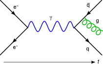
Feynman diagram
|
| History |
Although the unphysical axes in the space of detailed configurations are a fundamental property of the physical model, there is no special set of directions "perpendicular" to them. Hence there is an enormous amount of freedom involved in taking a "cross section" representing each physical configuration by a particular detailed configuration (or even a weighted distribution of them). Judicious gauge fixing can simplify calculations immensely, but becomes progressively harder as the physical model becomes more realistic; its application to quantum field theory is fraught with complications related to renormalization, especially when the computation is continued to higher orders. Historically, the search for logically consistent and computationally tractable gauge fixing procedures, and efforts to demonstrate their equivalence in the face of a bewildering variety of technical difficulties, has been a major driver of mathematical physics from the late nineteenth century to the present.[citation needed]
Contents
[hide]Gauge freedom[edit]
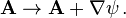
The archetypical gauge theory is the Heaviside–Gibbs formulation of continuum electrodynamics in terms of an electromagnetic four-potential, which is presented here in space/time asymmetric Heaviside notation. The electric field E and magnetic field B of Maxwell's equations contain only "physical" degrees of freedom, in the sense that every mathematical degree of freedom in an electromagnetic field configuration has a separately measurable effect on the motions of test charges in the vicinity. These "field strength" variables can be expressed in terms of the electric scalar potential and the magnetic vector potential A through the relations:
 (1)
(1)
 .
.
 .
.
 (2)
(2)
A particular choice of the scalar and vector potentials is a gauge (more precisely, gauge potential) and a scalar function ψ used to change the gauge is called a gauge function. The existence of arbitrary numbers of gauge functions ψ(r, t) corresponds to the U(1) gauge freedom of this theory. Gauge fixing can be done in many ways, some of which we exhibit below.
Although classical electromagnetism is now often spoken of as a gauge theory, it was not originally conceived in these terms. The motion of a classical point charge is affected only by the electric and magnetic field strengths at that point, and the potentials can be treated as a mere mathematical device for simplifying some proofs and calculations. Not until the advent of quantum field theory could it be said that the potentials themselves are part of the physical configuration of a system. The earliest consequence to be accurately predicted and experimentally verified was the Aharonov–Bohm effect, which has no classical counterpart. Nevertheless, gauge freedom is still true in these theories. For example, the Aharonov–Bohm effect depends on a line integral of A around a closed loop, and this integral is not changed by

No comments:
Post a Comment