"A 是固定
不變, 有水在管內流動與流速為F(x), 另外
由於管壁非完全封閉因此管壁四周同時也有
水滲入(或滲出), 我們想問的是此滲入率為
多少?(假設水的密度始終等於1) 我們取其中
一段[x, x+ x] 來看, 在單位時間內滲入到
這段管子的水量必須等於沿管子方向流出的
水量與流進的水量之差"
果
[PDF]Green定理與應用--林琦焜 - 數學系 - 國立成功大學
www.math.ncku.edu.tw/~fang/向量分析-Green定理與應用--林琦焜.pdfGreen定理與應用. 林琦焜. “數學沒有物理是瞎子, 物理沒有數學是跛子。” 1. 前言: 學習數學的經驗告訴自己“數學是很容. 易忘的” 這其中的原因乃是因為我們所學的
可微分函數, 且其梯度∇φ 為連續, ~r 為連接
~a,~b 兩點之任意曲線, 則
Z ~b
~a
∇φ · d~r = φ(~b) − φ(~a) (31)
這定理的物理意義(電學的角度): 沿著
電場上兩點間任一曲線電場所作的功為兩點
的電位差, 由Green 定理可知若F = ∇φ,
C1,C2 為連接~a,~b 之任意兩條曲線則
I
C
F · d~r =
Z
C1
F · d~r −
Z
C2
F · d~r
=
ZZ
R
∇ × (∇φ) · ~k dxdy = 0
因此Z
C1
F · d~r =
Z
C2
F · d~r
即線積分與路徑無關(path-independent),
~a,~b 兩點之任意曲線, 則
Z ~b
~a
∇φ · d~r = φ(~b) − φ(~a) (31)
這定理的物理意義(電學的角度): 沿著
電場上兩點間任一曲線電場所作的功為兩點
的電位差, 由Green 定理可知若F = ∇φ,
C1,C2 為連接~a,~b 之任意兩條曲線則
I
C
F · d~r =
Z
C1
F · d~r −
Z
C2
F · d~r
=
ZZ
R
∇ × (∇φ) · ~k dxdy = 0
因此Z
C1
F · d~r =
Z
C2
F · d~r
即線積分與路徑無關(path-independent),
[PDF]Green定理與應用--林琦焜 - 數學系 - 國立成功大學
www.math.ncku.edu.tw/~fang/向量分析-Green定理與應用--林琦焜.pdfStokes 定理與散度定理(Divergence The- orem) 則構成了應用數學的基礎。 2. 微積分基本定理: 微分與積分的關係這是微積分的主要房. 角石, 實際上這正是牛頓與萊 ...[PDF]數學(十四) Gauss定理與Stokes定理(續)
web.phys.ntu.edu.tw/ap/handout.../20050521math_note_second_14.pdf2005年5月21日 - Gauss定理與Stokes定理(續). •Gauss定理(另一種講法). 考慮中心點為r = (x,y,z)的小長方體(邊長為Ax,Ay,Az),流速場為v ( r)。流過前面的. 流量為.[PDF]第16 章向量微積分(Vector Calculus) 16.1 梯度, 旋度與散度 ...
case.ntu.edu.tw/CASTUDIO/Files/speech/Zip/CS0099S2B02_ch16.pdf16.5 Stokes 定理. . . . . . . . . . . . . . . . . . . . . . . . . . . . . . . 173. 16.1 梯度, 旋度與散度( Gradient, Curl and Divergence). 定義16.1.1. (1) 令f(x, y, z) 為純量場, 則其 ...[PDF]檔案下載
ocw.nctu.edu.tw/course/vanalysis/Green.pdfStokes 定理與散度定理(Divergence The- orem) 則Z成了應用數學的基礎。 2. «}基…ìÜ: 微分與積分的關係這是微積分的主要房. 角石, 實際上這正是牛頓與萊布尼茲 ...[PDF]pdf
msvlab.hre.ntou.edu.tw/grades/Engineering...100-2/.../Stokes定理.pdf2014 Stokes 定理.doc Y.C.Tu 製. Stokes 定理. Stokes 定理:. 1. 2. 1. 2. C. S. S. F tds. F n dS. F n dS. = ∇×. = ∇×. ∫. ∫∫. ∫∫. 其中,t 是ds 的單位切向量,n 是dS... Vector calculus - 海洋大學-力學聲響振動研究室
msvlab.hre.ntou.edu.tw/grades/Engineering-Mathematics...2/.../向量.htm... 2, 3 (程雋)) 機械系提問(doc)(pdf). 郭世榮老師解答(doc) (pdf) 卜偉晉推導 ... Green定理、Gauss定理 、Stokes定理 ... 2014 Stokes 定理(word)(pdf). Green-Stokes- ... [PDF]to download the PDF file. - 中研院數學研究所
w3.math.sinica.edu.tw/math_media/d352/35207.pdf這裡d 是對ζ 作用, 所以應用Stokes 定理, 立即可以得到Cauchy 積分公式。 於是從外微分形式的觀點, 問題便變成: 對於C2 中的區域Ω, 可否找到一個外微分形式.[PDF]微積分五講一一
w3.math.sinica.edu.tw/math_media/d302/30202.pdf同一公式表出來, 這個定理(或公式) 也叫做斯托克斯(Stokes) 定理(或Stokes 公式). ∫∂Ωω = ∫Ω dω. (2). 這裡, ω為外微分形式, dω為ω的外微分, Ω為dω的積分區域, ...[PDF]摘要複體組合學在拓撲,非線性分析,賽局論和數理經濟學中 ...
dspace.lib.ntnu.edu.tw/bitstream/77345300/59925/2/n089040002202.pdf由 陳建宏 著作 - 2008上組合型的Stokes定理,1993年施茂祥教授與李是男教授從幾何觀. 點發展一般位置映射,π平衡集、π次平衡集之相關理論,並且利用這. 些結果來證明在單純形上 ...[PDF]广义逆Stokes公式、广义逆Vening-Meinesz公式 ... - 中国科学
earth.scichina.com:8080/.../downloadArticleFile.do?...PDF... 轉為繁體網頁性由Stokes定理[1]和Dirichlet定理[3]所支持. 由(1)式定义的边值问题是已知扰动位T在边界. 面——球面上的值, 求边界面外的扰动位. 根据球的. 外部第一边值问题的 ...
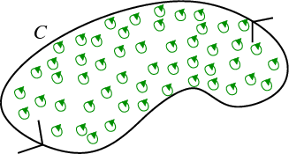
Stokes' theorem is a generalization of Green's theorem from circulation in a planar region to circulation along a surface. Green's theorem states that, given a continuously differentiable two-dimensional vector field
The “microscopic circulation” in Green's theorem is captured by the curl of the vector field and is illustrated by the green circles in the below figure.
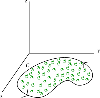
Green's theorem applies only to two-dimensional vector fields and to regions in the two-dimensional plane. Stokes' theorem generalizes Green's theorem to three dimensions. For starters, let's take our above picture and simply embed it in three dimensions. Then, our curve
The next question is what the microscopic circulation along a surface should be. For Green's theorem, we found that
In summary, to go from Green's theorem to Stoke's theorem, we've made two changes. First, we've changed the line integral living in two dimensions (Green's theorem) to a line integral living in three dimensions (Stokes' theorem). Second, we changed the double integral of
We write Stokes' theorem as:
Once we have Stokes' theorem, we can see that the surface integral of
For example, staring with a planar surface such as sketched above, we see that the surface
More information about applet.
Note that moving the green point on the top slider does not change the value of either integral in the above formulas. Since the curve
There is one more subtlety that you have to get correct, or else you'll may be off by a sign. You need to orient the surface and boundary properly. The cyan normal vector to the surface and the orientation of the curve (shown by red arrow) in the above applet are chosen with the proper relative orientations so that Stokes' theorem applies.
You can read some examples here.
https://www.ptt.cc/bbs/Physics/M.1253260265.A.193.html
http://mathinsight.org/circulation_unit_area_calculation
http://mathinsight.org/circulation_unit_area_calculation
curl F=0环路积分等于零 的結果 (無引號):
搜尋結果
旋度- 维基百科,自由的百科全书
zh.wikipedia.org/wiki/旋度
轉為繁體網頁沿着逆时针围绕漩涡的闭合曲线积分一定大于零,即是说环量大于零。这说明 ... 某个区域中的环量不等于零,说明这个区域中的向量场表现出环绕某一点或某一区域旋转的特性 :12。旋度则 ... 的旋度记作: \mathbf{curl\,}\mathbf{A} = \boldsymbol\ 从定义 .... \boldsymbol{\nabla} \times \mathbf{F}_2 =0. 所以 x>0 时是朝z轴负方向, x<0 ...
缺少字詞:路專供尚未註冊者使用討論區:這個保守場繞一圈,為什麼要消耗能量? - 格物 ...
www.phy.ntnu.edu.tw/demolab/phpBB/viewtopic.php?topic=22174
2009年8月4日 - 24 篇文章 - 5 位作者利用curl F = 0 就說F 是保守場,也是有條件的吧? (對位能的 ... 則curl F是零向量、環積分作功為零,而且直觀上正功和負功也抵消掉了,確實不作功.
區域D指的是由積分路經C所圍成的區域。 反之若 curlF=0,且區域D為單連通,則該積分值和路徑無關
※ 引述《ntust661 (Crm~)》之銘言: : curl(F) = 0 : 在任意一點 F 都存在 : 則可以稱F為保守場 這邊漏掉一個條件,除了在區域D中 F 可化為 gradf 外(也就是積分值和路徑無關), F及其一階偏導數在區域D中的每個點必須為連續函數 此時才能說curlF=0。而區域D指的是由積分路經C所圍成的區域。 反之若 curlF=0,且區域D為單連通,則該積分值和路徑無關。 : 那以下這個勒?! : -y x : F = ──── i + ──── j : x^2+y^2 x^2+y^2 : Curl(F) = 0 ? : 畫出圖形他是明顯的渦漩場 : 他竟然不能表示出任意點的環流密度!? : 我想知道的是,他沒環流密度(旋度)在(0,0)以外嗎? : 他不是保守場卻有保守場的特性 : 怪... 考慮一個線積分如下 → → ∮ F ˙dr 這個積分值等於多少會和你的積分路徑C有關 c c為任意的簡單封閉曲線,可分為兩類討論:< 1>積分路徑C不包含(0,0),則此時C路徑所圍成的區域D中 F恆滿足 curlF=0 for every point in "this" domain D 以及 對此D內的每個點而言,F及其一階偏導數皆連續 的這兩個條件 故curlF=0,所以只和起始點以及終點有關 因此積一圈必 = 0< 2>若一任意的積分路徑包含(0,0),則此時由C所形成的區域D 對 F來說顯然不是一個保守場!(因為D內並不是所有點都滿足保守場的兩個需求, 他只滿足 F=gradf,但(0,0)這點對F而言並不存在,當然就不連續) 因此積分值並不恆=0 又因為此時的積分路徑是任意的,所以就算你可以把該線積分grouping成 一個簡單的角度形式,你還是不知道答案是多少,如下 -ydx+xdy -1 y ∮ --------- = ∮ d(tan -) ,因為反三角函數是一多值函數,並不符合 c x^2+y^2 c x 微積分的要求。 但是我們可以透過取一個如下的路徑C*,使得C*所圍成的區域是一單連通區域 且藉此 「可將原題目中任意的路徑C變成一個我們想要的路徑(ex:圓)」 「且此時F在這個D*中為保守場」 有這兩個好處。 圖: http://0rz.tw/rlgsW 由圖可知 C* = C + AB + C1 + BA 且∫C* = ∫C+C1 (因為∫AB= -∫BA) 故得到 ∫C =∫C* - ∫C1 (a) 又因為剛剛所取的C*所圍成的區域是一個單連通區域,因為已知curlF=0 故對此不包含(0,0)的單連通區域而言,可以用Green's 定理,或由保守場, 皆可得 -ydx+xdy ∮ -------- = 0 (上述的好處之一) C* x^2+y^2 | 故由(a)可得 | ↓ -ydx+xdy -ydx+xdy ∮ -------- = 0 - ∮ -------- C x^2+y^2 C1 x^2+y^2 -1 y = ∮ d(tan -) -C1 x (-C1為逆時針) 這個時候因為路徑 -C1 已經明確了(一個圓形) 所以可以用極座標令 x=rcosθ,y=rsinθ (上述的好處之二) -1 y 且 r=(x^2+y^2)^(1/2),θ=tan - 且 θ:0~2π,此時的θ是單值函數 x 2π 因此所求 = ∮ dθ = ∫ dθ = 2π。 -C1 0 -- 簡單來說,保守場要連同路徑下去考慮,因為所謂的保守場就是 和路徑無關,因此所選取的簡單封閉曲線在哪是很重要的。也就是 如果簡單封閉曲線 不含 (0,0)則它具有保守場的特性,積一圈會=0 如果簡單封閉曲線 含 (0,0)則它不具有保守場的特性,積一圈不一定=0 (就算C沒有通過奇異點也是一樣) 你沒有考慮曲線C在哪,才會有他一下子是保守場一下子不是保守場的感覺。 -- 圖換過了 D*所在位置如圖所示 -- ※ 發信站: 批踢踢實業坊(ptt.cc) ◆ From: 114.40.86.251 ※ 編輯: Mpegwmvavi 來自: 114.40.77.252 (09/18 22:05)
推 ntust661:懂!大推! 09/18 23:06
→ ntust661:以前都會以為有源頭的場才可能是保守場 09/18 23:07
→ ntust661:例如重力場,靜電場 09/18 23:07
→ ntust661:原來這種也會是保守場 09/18 23:08
→ ntust661:繞一圈作功等於零 09/18 23:09
→ ntust661:在世界上,擁有這種場嗎? 09/18 23:09
推 justsaygood:考物研所的工數,這題會考... 也會叫你解釋是否保守 09/19 00:21
→ kevin60405:我在書上看到說 無限長直導線產生的磁場 就是這種場 09/19 02:20
推 ntust661:所以磁場就是保守場了... 09/19 02:21
→ kevin60405:arctan是多值函數?高中學他的值域不是在1.4象線嗎? 09/19 02:23
→ kevin60405:如此限制可以使它成為"函數" 而不是一對多 09/19 02:24
→ nightkid:arctan是多值函數 是人為定義讓他單值化 09/19 20:09
→ nightkid:還有 所謂函數是指一個x對應一個y arctan是符合的 09/19 20:09
→ kevin60405:我印象中多值函數不是不屬於函數嗎?
Math Insight
Calculating the formula for circulation per unit area
Given the definition for a component of the curl in the direction of a unit vector, we can sketch a proof for the formula of the “microscopic circulation” that we identify with curl. For simplicitiy, we will focus on the z -component of the curl, curlF⋅k , which is defined as
curlF(a)⋅k=lim A(C)→0 1A(C) ∫ C F⋅ds,
for a curve C around the point a=(a,b,c) in a plane that is parallel to the xy -plane. In the above limit, we let C shrink to a point so that the area A(C) inside C reduces to zero, as illustrated in the below applet. Since we divided by the area A(C) , we can interpret curl as being a “circulation per unit area.”
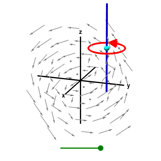 A line integral gives z-component of curl. A line integral around a curve in a plane perpendicular to the
 z -axis gives circulation of the vector field corresponding to the z -component of the curl. Dividing this line integral the the area of the region inside the curve, and letting the curve shrink to zero gives circulation per unit area. This circulation per unit area is the z -component of the curl. You can drag the red point on the slider to shrink the curve to a point.
More information about applet. The curve C is contained in the plane parallel to the xy -plane that passes through a , i..e., the plane given by z=c . In the integral, we can eliminate z by replacing it with the constant value c . Moreover, the tangent vectors along C must be parallel to the xy plane, which means their z -components will be zero. Since the line integral of a vector field integrates the tangent components of the vector field, the z -component of F will drop out of the integral ∫ C F⋅ds . Hence, we can, without loss of generality, replace our three-dimensional vector field F(x,y,z) with a two-dimensional vector field F(x,y) consisting of the first two components of the original F evaluated at z=c . We can then view the curve C as lying in the xy -plane.
Besides simplifying the notation, this change of perspective make explicit the fact that this calculation is also valid for calculating the “microscopic circulation” of two-dimensional vector fields, like we need for Green's theorem. We just need to remember that, by the right hand rule, positive values of the circulation correspond to counterclockwise rotation in thexy -plane.
The introductory pages give some intuition why the “circulation per unit area” of thez -component of the curl is
curlF⋅k=∂F 2 ∂x −∂F 1 ∂y .
Here we sketch a proof why
1A(C) ∫ C F⋅ds→∂F 2 ∂x −∂F 1 ∂y
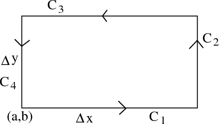
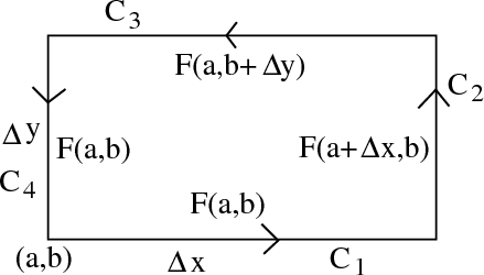
as we let C shrink to a point. Rather than use the circular C illustrated in the above applet, we let C be a rectangular curve, oriented counterclockwise. For simplicity of the notation, we'll let (a,b) be the lower-left point of C rather than being in the middle. Let the width and height of C be Δx and Δy , respectively. Label the edges of the rectangle by C 1 , C 2 , C 3 , and C 4 .
We assume the rectangle is small enough to approximateF as constant along each edge. Along the curve C 1 , the value of y is constantly b , but the value of x changes from a to a+Δx . We assume we can ignore that change in x (since the rectangle is small), and simply approximate F(x,y) as F(a,b) all along the segment C 1 .
Along the curveC 2 , the value of x is constantly a+Δx , but y changes from b to b+Δy . Since we assume we can ignore the change in y , we approximate F(x,y) as F(a+Δx,b) all along segment C 2 .
Similiarly, we approximateF(x,y) as F(a,b+Δy) all along segment C 3 and approximate F(x,y) as F(a,b) all along segment C 4 . We summarize these approximations in the following figure.
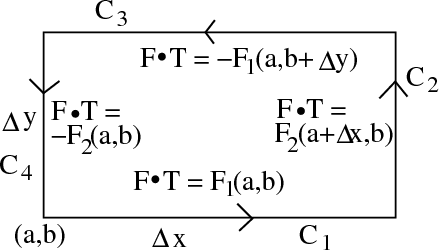
Next, to compute the integral∫ C F⋅ds , we remember that it is the same thing as integrating the scalar-valued function F⋅T , where T is the unit tangent vector along C :
∫ C F⋅ds=∫ C F⋅Tds.
We need to computeF⋅T along each segment of C . The tangent vector T is constant along each segment, and we are approximating F as constant along each segment, so the dot product F⋅T will be constant along each segment of C .
AlongC 1 , the path is directed in the positive x direction, so the unit tangent vector is T=(1,0) . The dot product F⋅T is simply the first component of F(a,b) :
F⋅T=F 1 (a,b).
AlongC 2 , the path is directed in the positive y direction, so T=(0,1) , and F⋅T is simply the second component of F(a+Δx,b) :
F⋅T=F 2 (a+Δx,b).
AlongC 3 , the path is directed in the negative x direction, so the unit tangent vector is T=(−1,0) . The dot product F⋅T is minus the first component of F(a,b+Δy) :
F⋅T=−F 1 (a,b+Δy).
AlongC 4 , the path is directed in the negative y direction, so T=(0,−1) , and F⋅T is minus the second component of F(a,b) :
F⋅T=−F 2 (a,b).
We summarize these findings in the following figure.
The integrals are now easy to compute. AlongC 1 , F⋅T is constant, so the integral is simply its value F 1 (a,b) times the length of the segment Δx :
∫ C 1 F⋅ds=∫ C 1 F⋅Tds=∫ C 1 F 1 (a,b)ds=F 1 (a,b)Δx.
Along C 2 , the integral is F 2 (a+Δx,b) times its length Δy :
∫ C 2 F⋅ds=F 2 (a+Δx,b)Δy.
Similarly,
∫ C 3 F⋅ds=−F 1 (a,b+Δy)Δx,
and
∫ C 4 F⋅ds=−F 2 (a,b)Δy.
The integral around all ofC is just the sum along the four segments
∫ C F⋅ds =∫ C 1 F⋅ds+∫ C 2 F⋅ds+∫ C 3 F⋅ds+∫ C 4 F⋅ds=F 1 (a,b)Δx+F 2 (a+Δx,b)Δy−F 1 (a,b+Δy)Δx−F 2 (a,b)Δy.
The circulation per unit area is the integral divided by the area of the rectangle, which isΔxΔy
∫ C F⋅dsΔxΔy =F 2 (a+Δx,b)Δy−F 2 (a,b)Δy−(F 1 (a,b+Δy)Δx−F 1 (a,b)Δx)ΔxΔy .
Half of the numerator is multiplied byΔy and half is multiplied byΔx . If we separate these into two fractions, we can cancel the Δy in the first fraction with the Δy in the demoninator
F 2 (a+Δx,b)Δy−F 2 (a,b)ΔyΔxΔy =F 2 (a+Δx,b)−F 2 (a,b)Δx .
In the second fraction, we can cancel theΔx ,
F 1 (a,b+Δy)Δx−F 1 (a,b)ΔxΔxΔy =F 1 (a,b+Δy)−F 1 (a,b)Δy .
Putting these back together, we have
∫ C F⋅dsΔxΔy =F 2 (a+Δx,b)−F 2 (a,b)Δx −F 1 (a,b+Δy)−F 1 (a,b)Δy .
Now, we let the curveC shrink down to a point. This means that Δx→0 and Δy→0 . In this limit, the two fractions become something familar: partial derivatives of F .
lim Δx,Δy→0 ∫ C F⋅dsΔxΔy =lim Δx→0 F 2 (a+Δx,b)−F 2 (a,b)Δx −lim Δy→0 F 1 (a,b+Δy)−F 1 (a,b)Δy =∂F 2 ∂x (a,b)−∂F 1 ∂y (a,b).
Therefore, the circulation per unit area around the point(x,y)=(a,b) is
∂F 2 ∂x (a,b)−∂F 1 ∂y (a,b).
This is the expression for the scalar curl that we use for the “microscopic circulation” in Green's theorem. If we rewrite this in terms of the original three-dimensional vector field F(x,y,z) at the point (x,y,z)=(a,b,c) , we obtain the expression for the z -component of the curl
curlF(a,b,c)⋅k=∂F 2 ∂x (a,b,c)−∂F 1 ∂y (a,b,c)
as promised.
More information about applet.
Besides simplifying the notation, this change of perspective make explicit the fact that this calculation is also valid for calculating the “microscopic circulation” of two-dimensional vector fields, like we need for Green's theorem. We just need to remember that, by the right hand rule, positive values of the circulation correspond to counterclockwise rotation in the
The introductory pages give some intuition why the “circulation per unit area” of the
We assume the rectangle is small enough to approximate
Along the curve
Similiarly, we approximate
Next, to compute the integral
We need to compute
Along
Along
Along
Along
We summarize these findings in the following figure.
The integrals are now easy to compute. Along
The integral around all of
The circulation per unit area is the integral divided by the area of the rectangle, which is
Half of the numerator is multiplied by
In the second fraction, we can cancel the
Now, we let the curve
Therefore, the circulation per unit area around the point
Thread navigation
Math 2374
Multivariable calculus
Notation systems
More information on notation systemsSimilar pages
- The idea behind Green's theorem
- The definition of curl from line integrals
- The idea behind Stokes' theorem
- The components of the curl
- A path-dependent vector field with zero curl
- Stokes' theorem examples
- Subtleties about curl
- Green's theorem with multiple boundary components
- Introduction to a line integral of a vector field
- The integrals of multivariable calculus
- More similar pages
No comments:
Post a Comment